Stochastic Dynamic Programming With Gaussian Process Approx

Here we work out an SDP solution of the Reed (1979) using a Gaussian process approximation. In this example the Gaussian process hyper-parameters haven’t been tuned, so in principle the solution would perform even better, but this is just for illustrative purposes.

We simulate 40 points under a stochastic growth (lognormal multiplicative noise) Beverton-Holt model and infer the Gaussian process. We start the simulation from a low stock value, giving reasonable but not perfect coverage of the state-space. The prior still has a strong influence outside these regions, so the GP doesn’t quite match the Beverton-Holt curve, as seen in the first figure.

We solve for the optimal policy function by discretizing the system and using the Gaussian process to fill out the stochastic transition matrix, which we pass to my little stochastic dynamic programming library to determine the policy function. We compare this policy function to the solution for the true F (Beverton-Holt) in the second figure, and note somewhat substantial differences (in particular a clear deviation from the constant escapement rule that emerges, which in itself is quite interesting, all though clearly non optimal in this case.

The GP doesn’t learn during the actual test period when the management is being implemented, though of course it could easily do so (after accounting for the application of the control). A single replicate simulation compares the optimal management under the true model to the GP management, which does less well (obviously), but not by a dramatic amount.

Code provides explicit statements of the models and should generate a reproducible example.

Next steps should optimize the GP and compare against the more realistic test case where the parameterized model is estimated from the simulation data (possibly under different functional forms, etc).

Coded example below, from reed-example.md

load my libraries and plotting lib.

require(nonparametricbayes)
require(pdgControl)
require(ggplot2)

(push images to flickr)

opts_knit$set(upload.fun = socialR::flickr.url)

Beverton-Holt function

Simulate some training data under a stochastic growth function with standard parameterization,

f <- BevHolt
p <- c(1.5, 0.05)
K <- (p[1] - 1)/p[2]

Parameter definitions

x_grid = seq(0, 1.5 * K, length = 101)
T <- 40
sigma_g <- 0.1
x <- numeric(T)
x[1] <- 1

Noise function, profit function

z_g <- function() rlnorm(1, 0, sigma_g)  #1+(2*runif(1, 0,  1)-1)*sigma_g #
profit <- profit_harvest(1, 0, 0)

Simulation

for (t in 1:(T - 1)) x[t + 1] = z_g() * f(x[t], h = 0, p = p)

Predict the function over the target grid

obs <- data.frame(x = x[1:(T - 1)], y = x[2:T])
X <- x_grid
library(nonparametricbayes)
gp <- gp_fit(obs, X, c(sigma_n = 0.5, l = 1.5))

Gaussian Process inference from this model. True model shown in red.

df <- data.frame(x = X, y = gp$Ef, ymin = (gp$Ef - 2 * sqrt(abs(diag(gp$Cf)))), 
    ymax = (gp$Ef + 2 * sqrt(abs(diag(gp$Cf)))))
true <- data.frame(x = X, y = sapply(X, f, 0, p))
require(ggplot2)
ggplot(df) + geom_ribbon(aes(x, y, ymin = ymin, ymax = ymax), fill = "gray80") + 
    geom_line(aes(x, y)) + geom_point(data = obs, aes(x, y)) + geom_line(data = true, 
    aes(x, y), col = "red", lty = 2)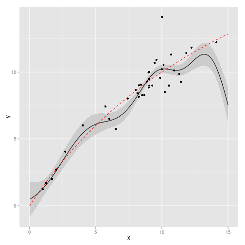

Stochastic Dynamic programming solution based on the posterior Gaussian process:

rownorm <- function(M) t(apply(M, 1, function(x) x/sum(x)))
h_grid <- x_grid

Define a transition matrix \(F\) from the Gaussian process, giving the probability of going from state \(x_t\) to \(x_{t+1}\). We already have the Gaussian process mean and variance predicted for each point \(x\) on our grid, so this is simply:

V <- sqrt(diag(gp$Cf))
matrices_gp <- lapply(h_grid, function(h) {
    F <- sapply(x_grid, function(x) dnorm(x, gp$Ef - h, V))
    F <- rownorm(F)
})

True \(f(x)\)

matrices_true <- lapply(h_grid, function(h) {
    mu <- sapply(x_grid, f, h, p)
    F_true <- sapply(x_grid, function(x) dnorm(x, mu, sigma_g))
    F_true <- rownorm(F_true)
})

Calculate the policy function using the true F:

opt_true <- find_dp_optim(matrices_true, x_grid, h_grid, 20, 0, profit, 
    delta = 0.01)

Calculate using the inferred GP

opt_gp <- find_dp_optim(matrices_gp, x_grid, h_grid, 20, 0, profit, 
    delta = 0.01)

require(reshape2)

policies <- melt(data.frame(stock = x_grid, GP = x_grid[opt_gp$D[, 
    1]], Exact = x_grid[opt_true$D[, 1]]), id = "stock")
q1 <- ggplot(policies, aes(stock, stock - value, color = variable)) + 
    geom_point() + xlab("stock size") + ylab("escapement")
q1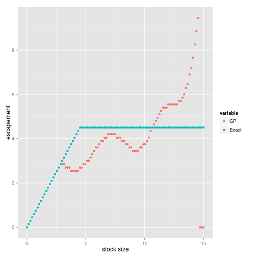

We can see what happens when we attempt to manage a stock using this:

z_g <- function() rlnorm(1, 0, sigma_g)

set.seed(1)
sim_gp <- ForwardSimulate(f, p, x_grid, h_grid, K, opt_gp$D, z_g, 
    profit = profit)
set.seed(1)
sim_true <- ForwardSimulate(f, p, x_grid, h_grid, K, opt_true$D, 
    z_g, profit = profit)

df <- data.frame(time = sim_gp$time, stock_gp = sim_gp$fishstock, 
    stock_true = sim_true$fishstock, harvest_gp = sim_gp$harvest, havest_true = sim_true$harvest)
df <- melt(df, id = "time")
ggplot(df) + geom_line(aes(time, value, color = variable))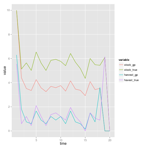

Total Profits

sum(sim_gp$profit)

## [1] 25.43

sum(sim_true$profit)

## [1] 29.95