Working out coded examples for basic Gaussian process regression using R. I’ve just read through the first few chapters of Rasmussen & Williams (2006), this implements the examples discussed in Chapter 2.1-2.5.
Required R libraries (for multivariate normal, also for plotting):
require(MASS)
require(reshape2)
require(ggplot2)
Set a seed for repeatable plots
set.seed(12345)Define the points at which we want to compute the function values (x values of the prediction points or test points), and the scale parameter for the covariance function \(\ell=1\)
x_predict <- seq(-5,5,len=50)
l <- 1
We will use the squared exponential (also called radial basis or Gaussian, though it is not this that gives Gaussian process it’s name; any covariance function would do) as the covariance function, \(\operatorname{cov}(X_i, X_j) = \exp\left(-\frac{(X_i - X_j)^2}{2 \ell ^ 2}\right)\)
SE <- function(Xi,Xj, l) exp(-0.5 * (Xi - Xj) ^ 2 / l ^ 2)
cov <- function(X, Y) outer(X, Y, SE, l)
COV <- cov(x_predict, x_predict)Generate a number of functions from the process
values <- mvrnorm(3, rep(0, length=length(x_predict)), COV)Reshape the data into long (tidy) form, listing x value, y value, and sample number
dat <- data.frame(x=x_predict, t(values))
dat <- melt(dat, id="x")
head(dat)
x variable value
1 -5.000 X1 -0.6450
2 -4.796 X1 -0.9227
3 -4.592 X1 -1.1587
4 -4.388 X1 -1.3277
5 -4.184 X1 -1.4139
6 -3.980 X1 -1.4103Plot the result
fig2a <- ggplot(dat,aes(x=x,y=value)) +
  geom_rect(xmin=-Inf, xmax=Inf, ymin=-2, ymax=2, fill="grey80") +
  geom_line(aes(group=variable)) +   theme_bw() +
  scale_y_continuous(lim=c(-3,3), name="output, f(x)") +
  xlab("input, x")
fig2a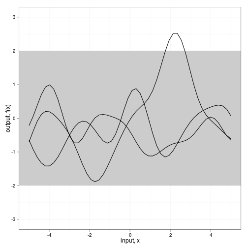
Posterior distribution given the data
Imagine we have some data,
obs <- data.frame(x = c(-4, -3, -1,  0,  2),
                  y = c(-2,  0,  1,  2, -1))
In general we aren’t interested in drawing from the prior, but want to include information from the data as well. We want the joint distribution of the observed values and the prior is:
\[\begin{pmatrix} y_{\textrm{obs}} \\ y_{\textrm{pred}} \end{pmatrix} \sim \mathcal{N}\left( \mathbf{0}, \begin{bmatrix} cov(X_o,X_o) & cov(X_o, X_p) \\ cov(X_p,X_o) & cov(X_p, X_p) \end{bmatrix} \right)\]
No observation noise
Assuming the data are known without error and conditioning on the data, and given \(x \sim \mathcal{N}(0, cov(X_o, X_o))\), then the conditional probability of observing our data is easily solved by exploiting the nice properties of Gaussians,
\[x|y \sim \mathcal{N}\left(E,C\right)\] \[E = cov(X_p, X_o) cov(X_o,X_o)^{-1} y\] \[C= cov(X_p, X_p) - cov(X_p, X_o) cov(X_o,X_o)^{-1} cov(X_o, X_p) \]
(We use solve(M) which with no second argument will simply invert the matrix M, but should use the Cholsky decomposition instead for better numerical stability)
cov_xx_inv <- solve(cov(obs$x, obs$x))
Ef <- cov(x_predict, obs$x) %*% cov_xx_inv %*% obs$y
Cf <- cov(x_predict, x_predict) - cov(x_predict, obs$x)  %*% cov_xx_inv %*% cov(obs$x, x_predict)
Now lets take 3 random samples from the posterior distribution,
values <- mvrnorm(3, Ef, Cf)and plot our solution (mean, 2 standard deviations, and the ranom samples.)
dat <- data.frame(x=x_predict, t(values))
dat <- melt(dat, id="x")

fig2b <- ggplot(dat,aes(x=x,y=value)) +
  geom_ribbon(data=NULL,
              aes(x=x_predict, y=Ef, ymin=(Ef-2*sqrt(diag(Cf))), ymax=(Ef+2*sqrt(diag(Cf)))),
              fill="grey80") +
  geom_line(aes(color=variable)) + #REPLICATES
  geom_line(data=NULL,aes(x=x_predict,y=Ef), size=1) + #MEAN
  geom_point(data=obs,aes(x=x,y=y)) +  #OBSERVED DATA
  scale_y_continuous(lim=c(-3,3), name="output, f(x)") +
  xlab("input, x")
fig2b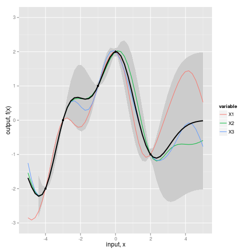
Additive noise
In general the model may have process error, and rather than observe the deterministic map \(f(x)\) we only observe \(y = f(x) + \varepsilon\). Let us assume for the moment that \(\varepsilon\) are independent, normally distributed random variables with variance \(\sigma_n^2\).
sigma.n <- 0.25
cov_xx_inv <- solve(cov(obs$x, obs$x) + sigma.n^2 * diag(1, length(obs$x)))
Ef <- cov(x_predict, obs$x) %*% cov_xx_inv %*% obs$y
Cf <- cov(x_predict, x_predict) - cov(x_predict, obs$x)  %*% cov_xx_inv %*% cov(obs$x, x_predict)
Now lets take 3 random samples from the posterior distribution,
values <- mvrnorm(3, Ef, Cf)and plot
dat <- data.frame(x=x_predict, t(values))
dat <- melt(dat, id="x")

fig2c <- ggplot(dat,aes(x=x,y=value)) +
  geom_ribbon(data=NULL,
              aes(x=x_predict, y=Ef, ymin=(Ef-2*sqrt(diag(Cf))), ymax=(Ef+2*sqrt(diag(Cf)))),
              fill="grey80") + # Var
  geom_line(aes(color=variable)) + #REPLICATES
  geom_line(data=NULL,aes(x=x_predict,y=Ef), size=1) + #MEAN
  geom_point(data=obs,aes(x=x,y=y)) +  #OBSERVED DATA
  scale_y_continuous(lim=c(-3,3), name="output, f(x)") +
  xlab("input, x")
fig2c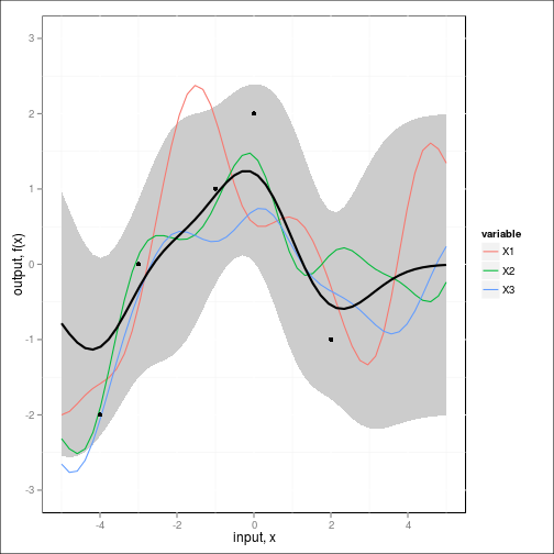
Note that unlike the previous case, the posterior no longer collapses completely around the neighborhood of the test points.
We can also compute the likelihood (and marginal likelihood over the prior) of the data directly from the inferred multivariate normal distribution, which can allow us to tune the hyperparameters such as the characteristic length scale \(\ell\) and the observation noise \(\sigma_n\). The most obvious approach would be to do so by maximum likelihood, giving point estimates of the hyper-parameters, though presumably we could be Bayesian about these as well.