No idea where I went wrong, but the final graphs are not what I expected Update: Integrated out some uncertainty in the expectation step, need to preserve full set of transtions

We consider adding additional sources of noise through observation error and implementation error to the orginal model of Reed (1979), which considers only growth error. This follows in the line of exploration taken by Clark and Kirkwood (1987), Roughgarden (1996) and Sethi (2006).

In adding these two sources of error, our state variable becomes our measured (or believed) stock \(x\), rather than the true stock size \(y\), and our control variable becomes the quota \(q\) set, rather than the realized harvest \(h\).

Analytical integrals

The central calculation to accomodating additional sources of uncertainty is the determination of the transition matrix; the probability of going from state \(x_t\) at time \(t\) to state \(x_{t+1}\) in the next interval, for each possible value of the control variable (quota). We discritize the statespace onto a fine grid of values \(x\) and \(h\) to seek a stochastic dynamic programming solution.

xmin <- 0
xmax <- 150
grid_n <- 100

We seek a harvest policy which maximizes the discounted profit from the fishery using a stochastic dynamic programming approach over a discrete grid of stock sizes from 0 to 150 on a grid of 100 points, and over an identical discrete grid of possible harvest values.

x_grid <- seq(xmin, xmax, length = grid_n)
h_grid <- x_grid

With purely growth noise, a row of the matrix is given by the probability density of the growth noise with mean \(f(x,h)\), that is, the probability of tranistion from \(x\) to \(x_{t+1}\) at harvest \(h\) is given by the function \(P(x_t+1, f(x,h))\) for some probability density function \(P\). In the case of uncertainty in stock \(y\) and harvest \(h\), we must integrate over the probability distributions for possible harvests and possible stock sizes,

In general this convolution can be non-trivial to compute, but in the case of uniformly distributed harvest error of \(\pm \sigma_i\) around some quota \(q\), and uniform measurement error of \(\pm \sigma_m\) around the true stock size \(x\), the integrals can be written as,

Note we enforce the simple non-negative boundary on stock and harvest.

So now we are left to merely integrate the \(f(y,h)\) over these finite intervals. We can do this for arbitrary \(f\) through multidimensional numerical integration (In fact we could have done this in the first place, but it is too slow for the convolutions of arbitrary probability densities)

int_f

function(f, x, q, sigma_m, sigma_i, pars){
  K <- pars[2]
  sigma_m <- K*sigma_m
  sigma_i <- K*sigma_i # scale noise into units of K
  
  if(sigma_m > 0 && sigma_i > 0){
    g <- function(X) f(X[1], X[2], pars)
    lower <- c(max(x - sigma_m, 0), max(q - sigma_i, 0))
    upper <- c(x + sigma_m, q + sigma_i)
    A <- adaptIntegrate(g, lower, upper)
    out <- A$integral/((q+sigma_i-max(q-sigma_i, 0))*(x+sigma_m-max(x-sigma_m, 0)))
  } else if(sigma_m == 0 && sigma_i > 0){ 
    g <- function(h) f(x, h, pars)
    lower <- max(q - sigma_i, 0)
    upper <- q + sigma_i
    A <- adaptIntegrate(g, lower, upper)
    out <- A$integral/(q+sigma_i-max(q-sigma_i, 0))
  } else if(sigma_i == 0 && sigma_m > 0){ 
    g <- function(y) f(y, q, pars)
    lower <- max(x - sigma_m, 0)
    upper <- x + sigma_m
    A <- adaptIntegrate(g, lower, upper)
    out <- A$integral/(x+sigma_m-max(x-sigma_m, 0))
  } else if (m == 0 && n == 0){
    out <- f(x,q,pars)
  } else {
    stop("distribution widths cannot be negative")
  }
  out
}
<environment: namespace:pdgControl>

If we assume a simple function like logistic growth, \(f(s) = r s (1-s/K) + s \), where \(s = x - h\),

f <- function(x, h, p) {
    sapply(x, function(x) {
        S = max(x - h, 0)
        p[1] * S * (1 - S/p[2]) + S
    })
}

With parameters

r <- 1
K <- 100
pars <- c(r, K)

r = 1 and K = 100.

Following Sethi et al, we can do this in closed form,

function(x,q, m, n, pars){
  K <- pars[2]
  m <- K*m
  n <- K*n # scale noise by K
  if(m > 0 && n > 0){
  out <- ((q+n-max(0,q-n))*(x+m-max(0,x-m))*(6*x*K-6*q*K-6*n*K+6*m*K+6*max(0,x-m)*K-6*
    max(0,q-n)*K-2*x^2+3*q*x+3*n*x-4*m*x-2*max(0,x-m)*x+3*max(0,q-n)*x-2*q^2-4*n*q+3*m*q+3*
    max(0,x-m)*q-2*max(0,q-n)*q-2*n^2+3*m*n+3*max(0,x-m)*n-2*max(0,q-n)*n-2*m^2-2*max(0,x-m)*m+3*
    max(0,q-n)*m-2*max(0,x-m)^2+3*max(0,q-n)*max(0,x-m)-2*max(0,q-n)^2))/(6*K)/((q+n-max(q-n, 0))*(x+m-max(x-m, 0)))
  } else if(m == 0 && n > 0) {
    y <- x
    out <- (((6*q+6*n-6*max(0,q-n))*y-3*q^2-6*n*q-3*n^2+3*max(0,q-n)^2)*K+(-3*q-3*n+3*max(0,q-n))*
      y^2+(3*q^2+6*n*q+3*n^2-3*max(0,q-n)^2)*y-q^3-3*n*q^2-3*n^2*q-n^3+max(0,q-n)^3)/(3*K*(q+n-max(q-n, 0)))
  } else if(n == 0 && m > 0){
    h <- q
    out <- ((3*x^2+(6*m-6*h)*x+3*m^2-6*h*m+6*max(0,x-m)*h-3*max(0,x-m)^2)*K-x^3+(3*h-3*m)*x^2+
      (-3*m^2+6*h*m-3*h^2)*x-m^3+3*h*m^2-3*h^2*m+3*max(0,x-m)*h^2-3*max(0,x-m)^2*h+max(0,x-m)^3)/(3*K*(x+m-max(x-m, 0)))
  } else if (m == 0 && n == 0){
    S <- max(x - q, 0)
    out <- S * (1 - S/K) + S
  } else {
    stop("distribution widths cannot be negative")
  }
  max(out,0)
}
<environment: namespace:pdgControl>

We can compare timing and equivalence of these two expressions:

require(cubature)
# Confirm that these give the same value, and time performance
system.time(a <- sapply(x_grid, function(x) int_f(f, x, 1, 0.1, 0.1, 
    pars)))

   user  system elapsed 
  7.444   0.000   7.394 

system.time(b <- sapply(x_grid, function(x) F(x, 1, 0.1, 0.1, pars)))

   user  system elapsed 
  0.012   0.000   0.015 

ggplot(data.frame(x = x_grid, a = a, b = b)) + geom_line(aes(x, a), 
    col = "red") + geom_line(aes(x, b), lty = 2)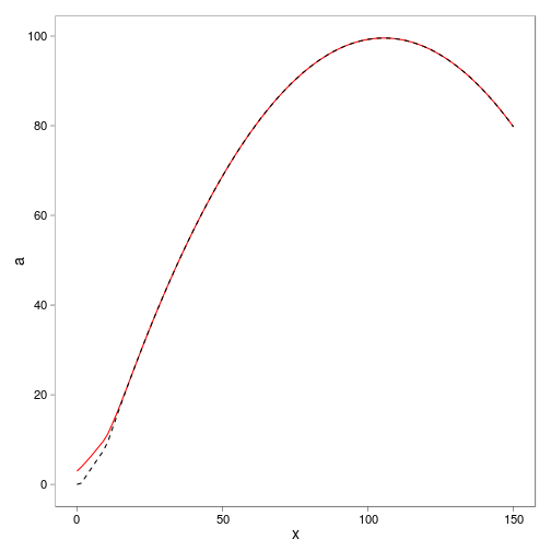

Note that as the uncertainy gets small, we recover the original transition probability \(f\):

F(50, 4, 0.1, 0.1, pars)

[1] 67.01

F(50, 4, 1e-04, 1e-04, pars)

[1] 70.84

f(50, 4, pars)

[1] 70.84

When the noise width is much smaller than the bin width we may have trouble, particularly with the uniform distribution, since part of the bin corresponds to zero density, part to high density.

Numerical implementation

We consider a profits from fishing to be a function of harvest h and stock size x, \( (x,h) = h - ( c_0 + c_1 ) \), conditioned on \( h > x \) and \(x > 0 \),

price <- 1
c0 <- 0
c1 <- 0
profit <- profit_harvest(price = price, c0 = c0, c1 = c1)

with price = 1, c0 = 0 and c1 = 0.

Additional parameters

delta <- 0.05
xT <- 0
OptTime <- 25
sigma_g <- 0.1
sigma_m <- 0.5
sigma_i <- 0.5

The uniform distribution must be careful for noise sizes smaller than binwidth

pdfn <- function(P, s) dunif(P, 1 - s, 1 + s)
# pdfn <- function(P, s) dlnorm(P, 0, s)

We will determine the optimal solution over a 25 time step window with boundary condition for stock at 0 and discounting rate of 0.05.

Scenarios:

sdp <- SDP_uniform(f, pars, x_grid, h_grid, sigma_g = sigma_g, pdfn, 
    sigma_m = sigma_m, sigma_i = sigma_i, F)

uniform <- find_dp_optim(sdp, x_grid, h_grid, OptTime, xT, profit, 
    delta, reward = 0)

Do the deterministic exactly,

SDP_Mat <- determine_SDP_matrix(f, pars, x_grid, h_grid, sigma_g = sigma_g, 
    pdfn)
det <- find_dp_optim(SDP_Mat, x_grid, h_grid, OptTime, xT, profit, 
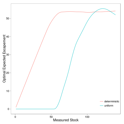
    delta, reward = 0)

Determine the policies for each of the scenarios (noise combinations).

plots

require(reshape2)
# policy <- melt(data.frame(stock = x_grid, deterministic=det$D[,1],
# uniform = uniform$D[,1], mc=opt$D[,1]), id = 'stock')
policy <- melt(data.frame(stock = x_grid, deterministic = det$D[, 
    1], uniform = uniform$D[, 1]), id = "stock")

ggplot(policy) + geom_jitter(aes(stock, stock - x_grid[value], color = variable), 
    shape = "+")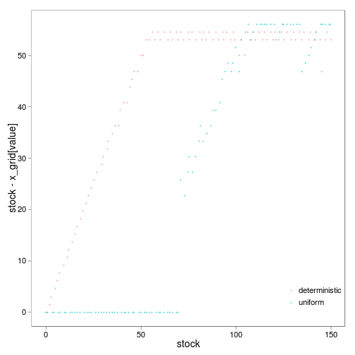

dat <- subset(policy, stock < 140)
dt <- data.table(dat)
linear <- dt[, approx(stock, stock - x_grid[value], xout = seq(1, 
    150, length = 15)), by = variable]
ggplot(linear) + stat_smooth(aes(x, y, color = variable), degree = 1, 
    se = FALSE, span = 0.3) + xlab("Measured Stock") + ylab("Optimal Expected Escapement")