Continuing writing and experimentation for examples in the warning signals manuscript, figuring out how to explain the need for the likelihood-based model comparison approach rather than the standard method of summary statistics.
The traditional approach computes a particular “leading indicator”, such as variance or autocorrelation, in a sliding window along the time series. If the system is loosing stability approaching a bifurcation, it’s leading eigenvalue must go through zero and hence shows critical slowing down, with the associated pattern of increasing autocorrelation an increasing variance.
Stating this trend isn’t the same as quantifying it statistically. What corresponds to an actual increase vs a random fluctuation? Typical approaches of the literature use a correlation test to check this. Unfortunately, the time series points aren’t independent, so the null expectation isn’t zero correlation. In fact, statistically significant correlation is observed in almost every simulation in which no warning signal is present: 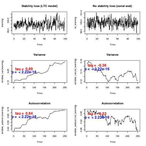
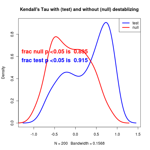
The tau parameter of Kendall’s correlation test should give some indication of the strength of trend. By simulating many times from both a null model and a relatively dramatic warning signal model, we see little correspondence between larger tau values and existence of the warning signal:
Despite the weakness of the leading indicators, these two signals should be quite distinguishable by likelihood:
# Likelihood Fits
> timedep <- updateGauss(timedep_LTC, pars=c(Ro=5, m=0, theta=100, sigma=1), warning, control=list(maxit=1000))
> const <- updateGauss(const_LTC, pars, warning, control=list(maxit=1000))
> llik_warning <- 2*(loglik(timedep)-loglik(const))

> timedep_no <- updateGauss(timedep_LTC, pars, no_warning, control=list(maxit=1000))
> const_no <- updateGauss(const_LTC, pars, no_warning, control=list(maxit=1000))
> llik_nowarning <- 2*(loglik(timedep_no)-loglik(const_no))

> llik_warning
[1] 18.95433
> llik_nowarning
[1] 0.882028