A quick foray into trying to understand why I see the wider distribution (though still symmetric) in the null of the OU model then in the null from the Allee model in the Prosecutor’s fallacy.
Load the original run of the ou model and increase the nulldt data frame to use all points instead of a sample of length 5000
load("beer_run.rda")

ou_dat <- dat
ou_null <- nulldat
#ou_null_ts <- nulldt

null <- timeseries #[1000:6010,]
null <- as.data.frame(cbind(time = 1:dim(null)[1], null))
ndf <- melt(null, id="time")
names(ndf) = c("time", "reps", "value")
levels(ndf$reps) <- 1:length(levels(ndf$reps)) # use numbers for reps instead of V1, V2, etc
nulldt <- data.table(ndf)
ou_null_ts <- nulldt
Plot the final distribution of indicator statistics, showing the width of the null,
ggplot(dat) + geom_histogram(aes(value, y=..density..), binwidth=0.3, alpha=.5) +
 facet_wrap(~variable) + xlim(c(-1, 1)) +
  geom_density(data=nulldat, aes(value), adjust=2) + xlab("Kendall's tau") + theme_bw()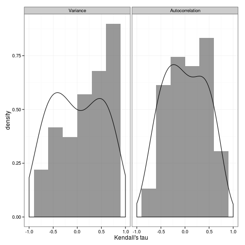
Load the allee model and rename variables appropriately,
load("comment_run.rda")
allee_dat <- dat
allee_null <- nulldat
allee_null_ts <- nulldt
For the Allee model, also plot the final distribution of indicator statistics, showing the width of the null,
ggplot(dat) + geom_histogram(aes(value, y=..density..), binwidth=0.3, alpha=.5) +
 facet_wrap(~variable) + xlim(c(-1, 1)) +
  geom_density(data=nulldat, aes(value), adjust=2) + xlab("Kendall's tau") + theme_bw()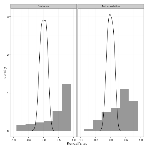
Tidy the data and plot a single replicate from each. Note the OU process has the correspondingly much wider null distribution due to
allee_x <- subset(allee_null_ts, reps==1)
ou_x <- subset(ou_null_ts, reps==1)
allee_x <- data.frame(time = allee_x$time, value = allee_x$value)
ou_x <- data.frame(time = ou_x$time, value = ou_x$value)

ggplot(allee_x, aes(time, value)) + geom_point()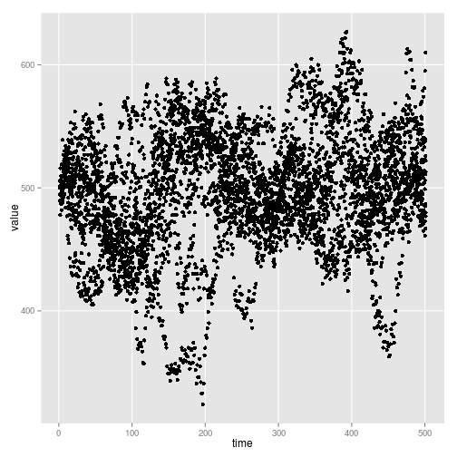
ggplot(ou_x, aes(time, value)) + geom_point()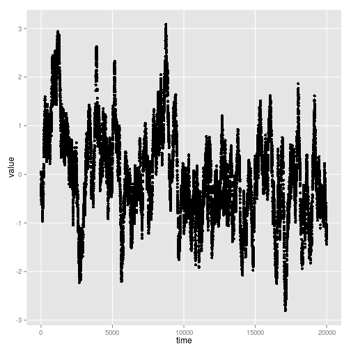
Note that subsampling the data at coarser interval doesn’t matter
warningtrend(ou_x[seq(1, length(ou_x$value),by=50),], window_var) tau
-0.5527 Nor does scaling matter (recall Kendall’s \(tau\) is a rank-correlation test)
warningtrend(data.frame(time=ou_x$time, value=(ou_x$value+1)*500), window_var) tau
-0.5516 warningtrend(data.frame(time=ou_x$time, value=ou_x$value), window_var) tau
-0.5516 Lengthening the sample suggests the sampling is not long enough to have converged in distribution of this statistic. Computing on this fine sampling resolution over adequate length of time quickly becomes prohibitive.
sapply(seq(1000, 20000, by=1000), function(i) warningtrend(ou_x[1:i,], window_var)) tau tau tau tau tau tau
0.1802475 -0.0832527 0.6365570 0.1787726 -0.1747774 -0.5295226
tau tau tau tau tau tau
-0.5403782 -0.6790710 -0.6114706 -0.2950858 -0.0444861 0.0006919
tau tau tau tau tau tau
-0.2579410 -0.5220490 -0.6439519 -0.6221482 -0.5545048 -0.5134236
tau tau
-0.5265975 -0.5515807