Load necessary libraries,
library(pdgControl)  # custom SDP functions
library(nonparametricbayes)  # custom
library(reshape2)  # data manipulation
library(data.table)  # data manipulation
library(plyr)  # data manipulation
library(ggplot2)  # plotting
library(tgp)  # Gaussian Processes
library(MCMCpack)  # Markov Chain Monte Carlo tools
library(R2jags)  # Markov Chain Monte Carlo tools
library(emdbook)  # Markov Chain Monte Carlo tools
library(coda)  # Markov Chain Monte Carlo tools
Plotting and knitr options, (can generally be ignored)
library(knitcitations)
opts_chunk$set(tidy = FALSE, warning = FALSE, message = FALSE, cache = FALSE)
opts_knit$set(upload.fun = socialR::flickr.url)
theme_set(theme_bw(base_size = 10))
theme_update(panel.background = element_rect(fill = "transparent",
    colour = NA), plot.background = element_rect(fill = "transparent", colour = NA))
cbPalette <- c("#000000", "#E69F00", "#56B4E9", "#009E73", "#F0E442",
    "#0072B2", "#D55E00", "#CC79A7")
Model and parameters
Uses the model derived in Allen et al, of a Ricker-like growth curve with an allee effect, defined in the pdgControl package,
f <- RickerAllee
p <- c(2, 10, 5)
K <- p[2]
allee <- p[3]
Various parameters defining noise dynamics, grid, and policy costs.
sigma_g <- 0.05
sigma_m <- 0.0
z_g <- function() rlnorm(1, 0, sigma_g)
z_m <- function() 1+(2*runif(1, 0,  1)-1) * sigma_m
x_grid <- seq(0, 1.5 * K, length=101)
h_grid <- x_grid
profit <- function(x,h) pmin(x, h)
delta <- 0.01
OptTime <- 20  # stationarity with unstable models is tricky thing
reward <- 0
xT <- 0
seed_i <- 111
Xo <- K # observations start from
x0 <- Xo # simulation under policy starts from
Tobs <- 35
Sample Data
obs <- sim_obs(Xo, z_g, f, p, Tobs=Tobs, nz=15,
                harvest = sort(rep(seq(0, .5, length=7), 5)), seed = seed_i)
Maximum Likelihood
alt <- par_est(obs,  init = c(r = p[1],
                              K = mean(obs$x[obs$x>0]),
                              s = sigma_g))
est <- par_est_allee(obs, f, p,
                     init = c(r = p[1] + 1,
                              K = p[2] + 2,
                              C = p[3] + 2,
                              s = sigma_g))
Non-parametric Bayes
#inv gamma has mean b / (a - 1) (assuming a>1) and variance b ^ 2 / ((a - 2) * (a - 1) ^ 2) (assuming a>2)
s2.p <- c(5,5)
tau2.p <- c(5,1)
d.p = c(10, 1/0.1, 10, 1/0.1)
nug.p = c(10, 1/0.1, 10, 1/0.1) # gamma mean
s2_prior <- function(x) dinvgamma(x, s2.p[1], s2.p[2])
tau2_prior <- function(x) dinvgamma(x, tau2.p[1], tau2.p[2])
d_prior <- function(x) dgamma(x, d.p[1], scale = d.p[2]) + dgamma(x, d.p[3], scale = d.p[4])
nug_prior <- function(x) dgamma(x, nug.p[1], scale = nug.p[2]) + dgamma(x, nug.p[3], scale = nug.p[4])
beta0_prior <- function(x, tau) dnorm(x, 0, tau)
beta = c(0)
priors <- list(s2 = s2_prior, tau2 = tau2_prior, beta0 = dnorm, nug = nug_prior, d = d_prior, ldetK = function(x) 0)
gp <- bgp(X=obs$x, XX=x_grid, Z=obs$y, verb=0,
meanfn="constant", bprior="b0", BTE=c(2000,20000,2),
m0r1=FALSE, corr="exp", trace=TRUE,
beta = beta, s2.p = s2.p, d.p = d.p, nug.p = nug.p, tau2.p = tau2.p,
s2.lam = "fixed", d.lam = "fixed", nug.lam = "fixed", tau2.lam = "fixed") hyperparameters <- c("index", "s2", "tau2", "beta0", "nug", "d", "ldetK")
posteriors <- melt(gp$trace$XX[[1]][,hyperparameters], id="index")
# Traces
ggplot(posteriors) + geom_line(aes(index, value)) + facet_wrap(~ variable, scale="free", ncol=1)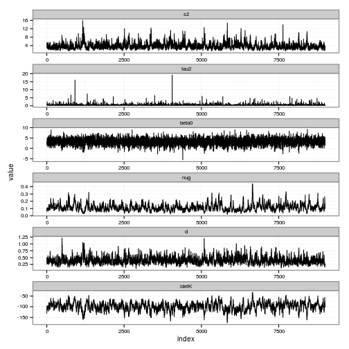
prior_curves <- ddply(posteriors, "variable", function(dd){
    grid <- seq(min(dd$value), max(dd$value), length = 100)
    data.frame(value = grid, density = priors[[dd$variable[1]]](grid))
})

#
ggplot(posteriors) + geom_histogram(aes(x=value, y=..density..), alpha=0.7) +
    geom_line(data=prior_curves, aes(x=value, y=density), col="red", lwd=2) +
    facet_wrap(~ variable, scale="free")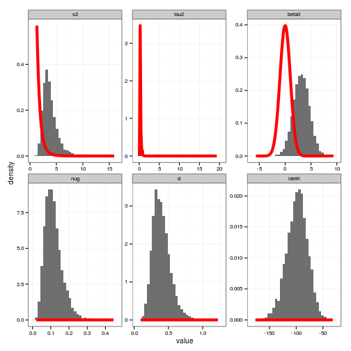
ggplot(posteriors, aes(value)) + stat_density(geom="path", position="identity", alpha=0.7) +
  geom_line(data=prior_curves, aes(x=value, y=density), col="red") +
  facet_wrap(~ variable, scale="free", ncol=2)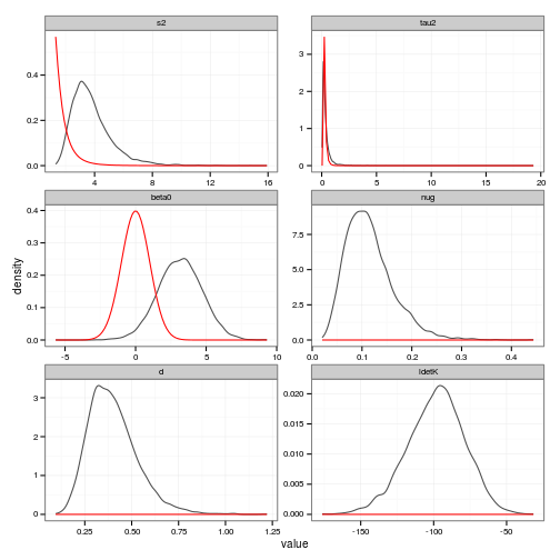
Parametric Bayes
We initiate the MCMC chain (init_p) using the true values of the parameters p from the simulation. While impossible in real data, this gives the parametric Bayesian approach the best chance at succeeding. y is the timeseries (recall obs has the \(x_t\), \(x_{t+1}\) pairs)
# a bit unfair to start with the correct values, but anyhow...
init_p = p
names(init_p) = c("r0", "K", "theta")
y <- obs$y[-1]
N=length(y);
We’ll be using the JAGS Gibbs sampler, a recent open source BUGS implementation with an R interface that works on most platforms. We initialize the usual MCMC parameters; see ?jags for details.
jags.data <- list("N","y")
n.chains = 1
n.iter = 20000
n.burnin = floor(n.iter/2)
n.thin = max(1, floor(n.chains * (n.iter - n.burnin)/1000))
The actual model is defined in a model.file that contains an R function that is automatically translated into BUGS code by R2WinBUGS. The file defines the priors and the model, as seen when read in here
cat(readLines(con="bugmodel-GammaPrior.txt"), sep="\n")## # Allen's Allee model based on a Ricker
##
## model{
##
## # Define prior densities for parameters
## K ~ dunif(1.0, 22000.0)
## logr0 ~ dunif(-4.0, 2.0)
## logtheta ~ dunif(-4.0, 2.0)
## iQ ~ dgamma(0.0001,0.0001)
## iR ~ dgamma(0.0001,0.0001)
##
## # Transform parameters to fit in the model
## r0 <- exp(logr0)
## theta <- exp(logtheta)
##
## # Initial state
## x[1] ~ dunif(0,10)
##
## # Loop over all states,
## for(t in 1:(N-1)){
## mu[t] <- x[t] + exp(r0 * (1 - x[t] / K) * (x[t] - theta) )
## x[t+1] ~ dnorm(mu[t],iQ)
## }
##
## # Loop over all observations,
## for(t in 1:(N)){
## y[t] ~ dnorm(x[t],iR)
## }
##
## }We define which parameters to keep track of, and set the initial values of parameters in the transformed space used by the MCMC. We use logarithms to maintain strictly positive values of parameters where appropriate. Because our priors on the noise parameters are inverse gamma distributed.
jags.params=c("K","logr0","logtheta","iR","iQ") # Don't need to save "x"
jags.inits <- function(){
  list("K"=init_p["K"],"logr0"=log(init_p["r0"]),"logtheta"=log(init_p["theta"]),"iQ"=1/0.05,"iR"=1/0.1,"x"=y,.RNG.name="base::Wichmann-Hill", .RNG.seed=123)
}
set.seed(12345)
time<-system.time(
  jagsfit <- jags(data=jags.data, inits=jags.inits, jags.params, n.chains=n.chains,
                  n.iter=n.iter, n.thin=n.thin, n.burnin=n.burnin,model.file="bugmodel-GammaPrior.txt")
)
## Compiling model graph
## Resolving undeclared variables
## Allocating nodes
## Graph Size: 394
##
## Initializing modeltime <- unname(time["elapsed"]);Convergence diagnostics for parametric bayes
jags_matrix <- as.data.frame(as.mcmc.bugs(jagsfit$BUGSoutput))
par_posteriors <- melt(cbind(index = 1:dim(jags_matrix)[1], jags_matrix), id = "index")

# Traces
ggplot(par_posteriors) + geom_line(aes(index, value)) + facet_wrap(~ variable, scale="free", ncol=1)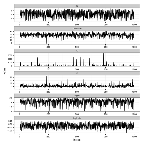
# posterior distributiosn
ggplot(par_posteriors, aes(value)) + stat_density(geom="path", position="identity", alpha=0.7) +
  facet_wrap(~ variable, scale="free", ncol=2)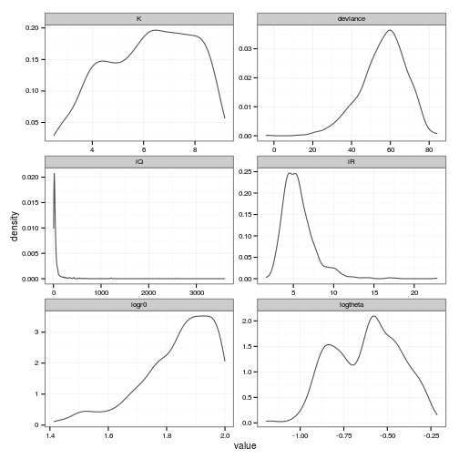
mcmc <- as.mcmc(jagsfit)
mcmcall <- mcmc[,-2]
who <- colnames(mcmcall)
who
## [1] "K" "iQ" "iR" "logr0" "logtheta"mcmcall <- cbind(mcmcall[,1],mcmcall[,2],mcmcall[,3],mcmcall[,4],mcmcall[,5])
colnames(mcmcall) <- whoPhase-space diagram of the expected dynamics
gp_plot(gp, f, p, est$f, est$p, alt$f, alt$p, x_grid, obs, seed_i)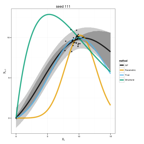
Optimal policies by value iteration
Compute the optimal policy under each model using stochastic dynamic programming.
MaxT = 1000
matrices_gp <- gp_transition_matrix(gp$ZZ.km, gp$ZZ.ks2, x_grid, h_grid)
opt_gp <- value_iteration(matrices_gp, x_grid, h_grid, MaxT, xT, profit, delta, reward)

matrices_true <- f_transition_matrix(f, p, x_grid, h_grid, sigma_g)
opt_true <- value_iteration(matrices_true, x_grid, h_grid, OptTime=MaxT, xT, profit, delta=delta)

matrices_estimated <- f_transition_matrix(est$f, est$p, x_grid, h_grid, est$sigma_g)
opt_estimated <- value_iteration(matrices_estimated, x_grid, h_grid, OptTime=MaxT, xT, profit, delta=delta)

matrices_alt <- f_transition_matrix(alt$f, alt$p, x_grid, h_grid, alt$sigma_g)
opt_alt <- value_iteration(matrices_alt, x_grid, h_grid, OptTime=MaxT, xT, profit, delta=delta)


pardist <- mcmcall
pardist[,4] = exp(pardist[,4]) # transform model parameters back first
pardist[,5] = exp(pardist[,5])


matrices_par_bayes <- parameter_uncertainty_SDP(f, p, x_grid, h_grid, pardist)
opt_par_bayes <- value_iteration(matrices_par_bayes, x_grid, h_grid, OptTime=MaxT, xT, profit, delta=delta)


OPT = data.frame(GP = opt_gp$D, True = opt_true$D, MLE = opt_estimated$D, Ricker.MLE = opt_alt$D, Parametric.Bayes = opt_par_bayes$D)
colorkey=cbPalette
names(colorkey) = names(OPT)
Graph of the optimal policies
policies <- melt(data.frame(stock=x_grid, sapply(OPT, function(x) x_grid[x])), id="stock")
names(policies) <- c("stock", "method", "value")
ggplot(policies, aes(stock, stock - value, color=method)) +
  geom_line(lwd=1.2, alpha=0.8) + xlab("stock size") + ylab("escapement")  +
  scale_colour_manual(values=colorkey)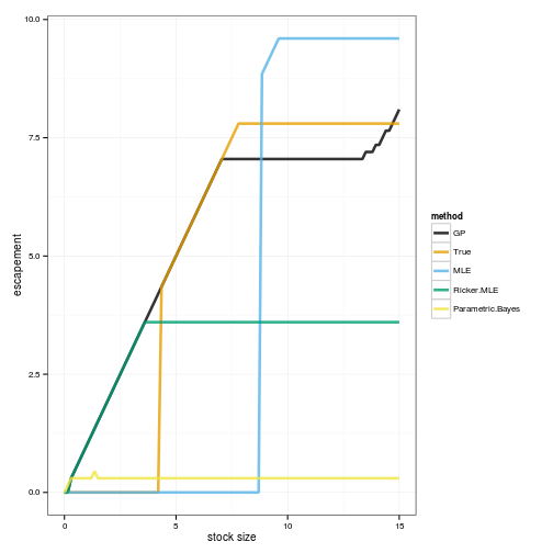
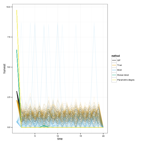
Simulate 100 realizations managed under each of the policies
sims <- lapply(OPT, function(D){
  set.seed(1)
  lapply(1:100, function(i)
    ForwardSimulate(f, p, x_grid, h_grid, x0, D, z_g, profit=profit, OptTime=OptTime)
  )
})


dat <- melt(sims, id=names(sims[[1]][[1]]))
dt <- data.table(dat)
setnames(dt, c("L1", "L2"), c("method", "reps"))
# Legend in original ordering please, not alphabetical:
dt$method = factor(dt$method, ordered=TRUE, levels=names(OPT))

ggplot(dt) +
  geom_line(aes(time, fishstock, group=interaction(reps,method), color=method), alpha=.1) +
  scale_colour_manual(values=colorkey, guide = guide_legend(override.aes = list(alpha = 1)))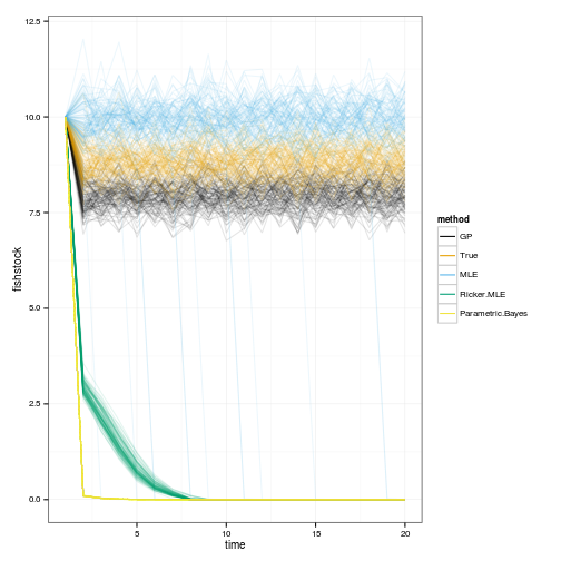
ggplot(dt) +
  geom_line(aes(time, harvest, group=interaction(reps,method), color=method), alpha=.1) +
  scale_colour_manual(values=colorkey, guide = guide_legend(override.aes = list(alpha = 1)))