Bayesian Parametric Uncertainty Sdp

Adapting the parametric uncertainty represented by the posterior distributions of the Bayesian estimate (see earlier notes) to the stochastic dynamic programming solution for the optimal policy. Simply requires evaluating the expectation over the distribution, but is computationally intensive given the spread and the three parameters.

f_transition_matrix <- function(f, p, x_grid, h_grid, sigma_g, pardist){
  lapply(h_grid, par_F, f, p, x_grid, sigma_g, pardist)
}


par_F <- function(h, f, p, x_grid, sigma_g, pardist, n_mc = 100){
  
  # Set up monte carlo sampling 
  d <- dim(pardist)
  indices <- round(runif(n_mc,1, d[1]))
  
  # Compute the matrix
  F_true <- 
    sapply(x_grid, function(x_t){           # For each x_t  

      bypar <- sapply(indices, function(i){ # For each parameter value
        p <- unname(pardist[i,c(4,1,5)])    # parameters for the mean, at current sample 
        mu <- f(x_t,h,p)
        est_sigma_g <- pardist[i,2]         # Variance parameter 

        if(snap_to_grid(mu,x_grid) < x_grid[2]){ # handle the degenerate case 
          out <- numeric(length(x_grid))
          out[1] <- 1
          out
        } else {
          out <- dlnorm(x_grid/mu, 0, est_sigma_g) 
        }
      })  
      ave_over_pars <- apply(bypar, 1, sum) # collapse by weighted average over possible parameters    
      ave_over_pars / sum(ave_over_pars)
      })
  F_true <- t(F_true)
        
}


snap_to_grid <- function(x, grid) sapply(x, function(x) grid[which.min(abs(grid - x))])   


# internal helper function
rownorm <- function(M) 
  t(apply(M, 1, function(x){ 
    if(sum(x)>0){
      x/sum(x)
    } else {
      out <- numeric(length(x))
      out[1] <- 1
      out
    }
  }))

Run the Bayesian analysis to obtain posterior distributions for parameters.

Test case using perturbed parameters

First, sanity test. Use the correct parameter values (slightly perturbed).

pardist <- mcmcall
pardist[,1] = p[2] + rnorm(100, 0, 0.000001)
pardist[,4] = p[1] + rnorm(100, 0, 0.000001)
pardist[,2] = sigma_g + rnorm(100, 0, 0.000001)
pardist[,5] = p[3] + rnorm(100, 0, 0.000001)

Compute optimal policy

sdp = f_transition_matrix(f, p, x_grid, h_grid, sigma_g, pardist)
s_opt <- value_iteration(sdp, x_grid, h_grid, OptTime=1000, xT, profit, delta)

Compare to the case without parameter uncertainty (growth noise only)

SDP_Mat <- determine_SDP_matrix(f, p, x_grid, h_grid, sigma_g)
pars_fixed <- value_iteration(SDP_Mat, x_grid, h_grid, OptTime=1000, xT, profit, delta)

Plot results

require(reshape2)
policies <- melt(data.frame(stock=x_grid, pars.uncert = x_grid[s_opt$D], pars.fixed = x_grid[pars_fixed$D]), id="stock")
ggplot(policies, aes(stock, stock - value, color=variable)) + geom_line(alpha=1) + xlab("stock size") + ylab("escapement")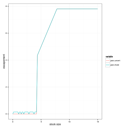 

Using actual estimates

pardist <- mcmcall

Transform parameters back

pardist[,4] = exp(pardist[,4])
pardist[,5] = exp(pardist[,5])

Compute optimal policy

sdp = f_transition_matrix(f, p, x_grid, h_grid, sigma_g, pardist)
s_opt <- value_iteration(sdp, x_grid, h_grid, OptTime=1000, xT, profit, delta)

Compare to the case without parameter uncertainty (growth noise only)

SDP_Mat <- determine_SDP_matrix(f, p, x_grid, h_grid, sigma_g)
pars_fixed <- value_iteration(SDP_Mat, x_grid, h_grid, OptTime=1000, xT, profit, delta)

Plot results

require(reshape2)
policies <- melt(data.frame(stock=x_grid, pars.uncert = x_grid[s_opt$D], pars.fixed = x_grid[pars_fixed$D]), id="stock")
ggplot(policies, aes(stock, stock - value, color=variable)) + geom_line(alpha=1) + xlab("stock size") + ylab("escapement")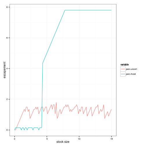 

To Do

So far this is just a proof of principle example.

• Needs to be adjusted to account for uncertainty in the estimates of the noise processes as well.
• Needs to be written as generic and documented functions, add to nonparametric-bayes package routines.