Parametric Bayesian Example

As discussed with Marc in yesterday’s meeting, it would be useful to compare the Gaussian process, as a nonparametric Bayesian estimate, to the optimal management solution under a parametric Bayesian case, e.g. with the correct underlying model. This is implemented in BUGS (jags) through the R interface as described in Bolker B, Gardner B, Maunder M, Berg C, Brooks M, Comita L, Crone E, Cubaynes S, Davies T, de Valpine P, Ford J, Gimenez O, Kery M, Kim E, Lennert-Cody C, Magnusson A, Martell S, Nash J, Nielsen A, Regetz J, Skaug H and Zipkin E (2013). “Strategies For Fitting Nonlinear Ecological Models in R, ad Model Builder, And Bugs.” Methods in Ecology And Evolution, pp. n/a–n/a. .“>Bolker et. al. (2013) , and follows the state-space model analysis along the lines outlined in Pedersen et. al. (2011) .

We base the estimate on the same simulated data as for the GP and MLE approaches,

f <- RickerAllee
p <- c(2, 10, 5)
K <- 10
allee <- 5

with the same parameters (many of which we won’t need until the SDP value iteration),

sigma_g <- 0.05
sigma_m <- 0
z_g <- function() rlnorm(1, 0, sigma_g)
z_m <- function() 1 + (2 * runif(1, 0, 1) - 1) * sigma_m
x_grid <- seq(0, 1.5 * K, length = 101)
h_grid <- x_grid
profit <- function(x, h) pmin(x, h)
delta <- 0.01
OptTime <- 20  # stationarity with unstable models is tricky thing
reward <- 0
xT <- 0
seed_i <- 1
Xo <- K  # observations start from
x0 <- Xo  # simulation under policy starts from
Tobs <- 35

Generate the simulated data

obs <- sim_obs(Xo, z_g, f, p, Tobs = Tobs, nz = 1, harvest = sort(rep(seq(0, 
    0.5, length = 7), 5)), seed = seed_i)

And fit the MLE models as before

alt <- par_est(obs, init = c(r = p[1], K = mean(obs$x[obs$x > 0]), 
    s = sigma_g))
est <- par_est_allee(obs, f, p, init = c(r = p[1] + 1, K = p[2] + 
    2, C = p[3] + 2, s = sigma_g))

Parametric Bayesian model fit

We will use the jags interface from R,

library(R2jags)

initialize parameters. The parametric equation (in this case, matching the true dynamics) and priors are defined in BUGS notation in text file.

init_p = est$p
names(init_p) = c("r0", "K", "theta")
y <- obs$y[-1]
N = length(y)

jags.data <- list("N", "y")
n.chains = 1
n.iter = 20000
n.burnin = floor(n.iter/2)
n.thin = max(1, floor(n.chains * (n.iter - n.burnin)/1000))

JAGS using gamma priors on precision

jags.params=c("K","logr0","logtheta","iR","iQ"); # Don't need to save "x"
jags.inits <- function(){
  list("K"=init_p["K"],"logr0"=log(init_p["r0"]),"logtheta"=log(init_p["theta"]),"iQ"=1/0.05,"iR"=1/0.1,"x"=y,.RNG.name="base::Wichmann-Hill", .RNG.seed=123)
}
set.seed(12345)
time<-system.time(       
  jagsfit <- jags(data=jags.data, inits=jags.inits, jags.params, n.chains=n.chains, 
                  n.iter=n.iter, n.thin=n.thin, n.burnin=n.burnin,model.file="bugmodel-GammaPrior.txt")
)         

time <- unname(time["elapsed"]);

Summarize the results

library(emdbook)
library(coda)
tfit_jags_m <- as.mcmc.bugs(jagsfit$BUGSoutput)
print(xyplot(tfit_jags_m))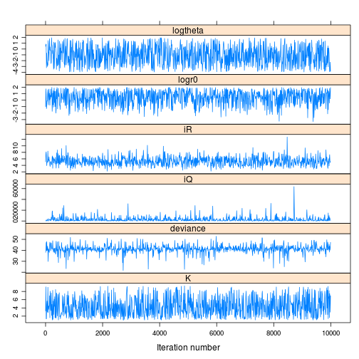

print(densityplot(tfit_jags_m))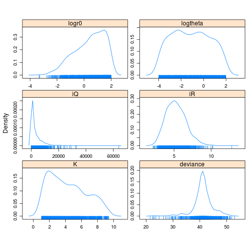

We collect model parameters over the replicate runs,

mcmc <- as.mcmc(jagsfit)
mcmcall <- mcmc[, -2]
who <- colnames(mcmcall)
mcmcall <- cbind(mcmcall[, 1], mcmcall[, 2], mcmcall[, 3], mcmcall[, 
    4], mcmcall[, 5])
colnames(mcmcall) <- who

Further parameter exploration

We will need to integrate over parameter uncertainty. Can consider the discritized binning

theta <- exp(mcmcall[, "logtheta"])
theta_dist <- hist(theta, freq = FALSE)

theta_dist$mids

##  [1] 0.25 0.75 1.25 1.75 2.25 2.75 3.25 3.75 4.25 4.75 5.25 5.75 6.25 6.75
## [15] 7.25

theta_dist$density

##  [1] 1.154 0.256 0.130 0.092 0.068 0.058 0.044 0.042 0.042 0.018 0.022
## [12] 0.026 0.022 0.014 0.012

delta <- theta_dist$mids[2] - theta_dist$mids[1]

Evaluating the value function given \(f\) fixed at each of theta_dist$mids multiplied by theta_dist$density * delta and summed over each \(\theta\) is going to be slow for a single parameter but simply unrealistic for higher dimensions.

References

• Benjamin M. Bolker, Beth Gardner, Mark Maunder, Casper W. Berg, Mollie Brooks, Liza Comita, Elizabeth Crone, Sarah Cubaynes, Trevor Davies, Perry de Valpine, Jessica Ford, Olivier Gimenez, Marc Kery, Eun Jung Kim, Cleridy Lennert-Cody, Arni Magnusson, Steve Martell, John Nash, Anders Nielsen, Jim Regetz, Hans Skaug, Elise Zipkin, (2013) Strategies For Fitting Nonlinear Ecological Models in R, ad Model Builder, And Bugs. Methods in Ecology And Evolution n/a-n/a 10.1111/2041-210X.12044
• M.W. Pedersen, C.W. Berg, U.H. Thygesen, A. Nielsen, H. Madsen, (2011) Estimation Methods For Nonlinear State-Space Models in Ecology. Ecological Modelling 222 1394-1400 10.1016/j.ecolmodel.2011.01.007