Ran a introductory tutorial on birth-death models for phylogenetic trees in R today for Peter Wainwright’s section of the Pop Bio Core sequence. Notes below, in a manner that may suggest I was better organized than reality might attest. Luckily the firsties are brilliant…
Getting Started
Code is shown section by section with results in the following examples. If you prefer, you can download my full code file here, but you will have to comment out my flickr plotting utilities before it will run. Here we go:
Install and load the packages “TreeSim” and “laser”. Will require a recent version of R for TreeSim to install correctly. We also write two simple custom functions to make our life easier, one to get the age of a tree, one to solve r= b-d and a= b/d for b and d.
install.packages(c("TreeSim", "laser"))
require(TreeSim); require(laser)

## tree age
treeage <- function(tree){
  if(is(tree, "phylo")){
    tree <- ape2ouch(tree, scale=FALSE)
    time <- max(tree@times)
  } else {
    time <- 0
  }
  time
}

# r is diversification rate, b-d, and a is d/b
# we'd rather have in terms of b and d
swp <- function(r, a){
  b = r/(1-a)
  d = r*a/(1-a)
  c(b,d)
}
Simulating Birth-Death Trees
We’ll start with the TreeSim function sim.bd.age to create birth-death trees. These examples illustrate the diversity of possible outcomes that result from the identical model. They also highlight subtleties in defining a model – such as, “was that the age from the origin, or the mrca?” Our first tree: ((yeah, so this tutorial isn’t that introductory – check the help file on sim.bd.age if you’ve forgotten what the arguments to the function are. We assume knowledge of R b.c. students have used it all year now.))
set.seed(0) # so we all get the same result
tree <- sim.bd.age(age=2,numbsim=1,lambda=2,mu=0,comp=F, mrca=F)
print( treeage(tree[[1]])  )
We get age=1.907982. Less than the age 2 we asked for, as Tomomi had pointed out. This means the founder species took about 0.1 time steps before the first speciation event. We expect the waiting times to be exponentially distributed. This is easy to confirm:
set.seed(0) # so we all get the same result
  trees <- sim.bd.age(age=2,num=100,lambda=2,0,comp=F, mrca=F)
  times <- sapply(trees, function(tr){
    2 - treeage(tr)
  })
  times <- times[times!=2] # trees that never branch don't contribute
## Plot Results
hist(times, freq=F)
curve(dexp(x, 2), add=T) # theory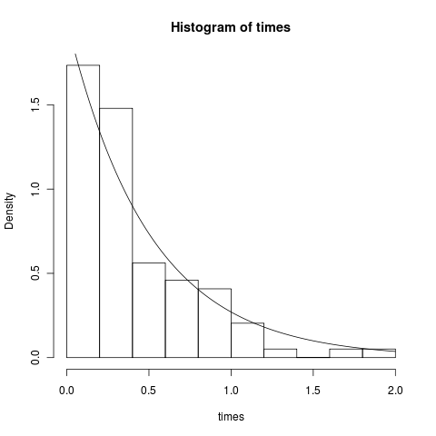
As we mentioned, setting the age equal to the most recent common ancestor (mrca) means the tree does have the age specified. We wondered if this held true when the tree had extinction, since it is possible the first branching event could end up with no descendants on one branch. In that case it isn’t the mrca of extant taxa, and it gets pruned, such that the total length of the tree is still the age given. ((So if we show the complete tree (complete=TRUE) with extinct taxa, is such a taxon floating or lost?)) This example tests this a bunch of times:
  ## This tree is exactly the age we asked for:
  tree <- sim.bd.age(2,1,2,0,complete=F, mrca=T)
  print(  treeage( tree[[1]] )  )

  ## This tree isn't always the age we asked for, or is it:
  trees <- sim.bd.age(2,20,5,4.9,comp=T, mrca=T)
  print(  sapply(trees, function(tr) treeage(tr))   )
Okay, onto visualizing differences in simulation outcomes. The most obvious is the variety in tip counts, as seen in this 6 taxon example:
  trees <- sim.bd.age(age=2,numbsim=6,lambda=2,mu=.5,mrca=TRUE,complete=FALSE)
  par(mfrow=c(3,2))
  for(i in 1:6)
    plot(trees[[i]])
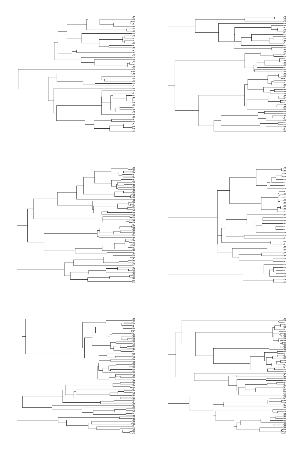
Do trees that branch early tend to be the ones with more species?
Notice these trees tend to have many more species than if we were to have mrca=FALSE, because they are older. Conditioning on MRCA age also means that we don’t see empty trees, like we do when we specify age since origin:
Recall we expect: \[ e^{\lambda t} \approx 54 \] tips on average., and in the case of MRCA=true:
   tips <- sapply(trees,
                  function(x){
                    if(!is(x, "phylo"))
                      ans <- 0  ## If the object isn't a tree, it's `cause all extinct
                   else
                     ans <- x$Nnode+1 ## num tip taxa = 1+internal nodes                    ans}) > ## R OUTPUT
> tips
[1] 49 53 70 40 71 64
> exp(4) ## expectation
[1] 54.59815
> mean(tips)  ## observed over 6 replicates
[1] 57.83333
Running more replicates we can see the long tail of the Poisson. 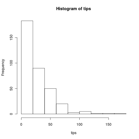
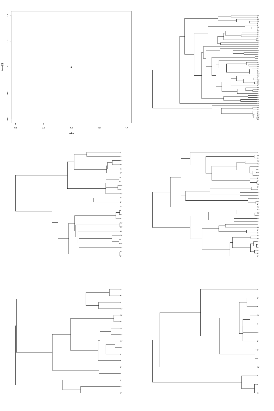
Conditioning on number of taxa
Often we are not interested in all possible trees (X), but only the subset that have the observed number (N) of taxa. This results from conditioning on N:
\[ P(X) = P(X|N)P(N) \]
Generating our trees with this command instead accomplishes that. For a great discussion of these issues see the TreeSim paper (Stadler, 2011)
trees<- sim.bd.taxa(n=20,numbsim=6,lambda=2,mu=.5,complete=FALSE)[[1]]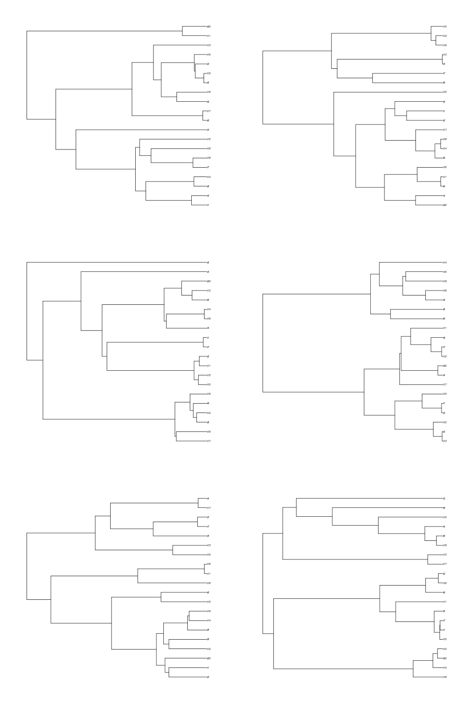
Fitting Models
### Let's take a closer look at estimating parameters from trees now.   ###
## Start with a simple tree
  tree <- sim.bd.age(age=2,numbsim=1,lambda=2,mu=0.0, mrca=FALSE,complete=FALSE)[[1]]
# fit a birth death model
# gives confidence levels that assume normality
  birthdeath(tree)
## laser's way of estimating a model
  model <- bd(branching.times(tree))
## estimate a yule model
  yule <- pureBirth(branching.times(tree))
# which one is better
  model$aic - yule$aic
Bootstrapping Models
# simulate a tree, fit a birth-death model, pull out the b and d parameters
  tree <- sim.bd.age(age=4,numbsim=1,lambda=2,mu=0.9,
                      mrca=FALSE,complete=FALSE)[[1]]
  fit <- bd(branching.times(tree))
  para <- swp(fit$r, fit$a)
# simulate lots of trees
  boots <- sim.bd.age(age=2, numbsim=500, lambda=para[1], mu=para[2],
                      mrca=FALSE, comp=FALSE)
  bd_dist <- sapply(boots,
              function(x){
                fit <- try(bd(branching.times(x)))
  ## Some fits fail because bd sucks too.  tell R to tough it out anyhow
                if(!is(fit, "try-error"))
                  para <- swp(fit$r, fit$a)
                else
                  para <- NA
                c(para[1], para[2])
              })
  ## err, fix formatting if sapply failed to give me a matrix!
  if(is(bd_dist, "list"))
    bd_dist <- sapply(1:length(bd_dist),
      function(i) c(bd_dist[[i]][1],bd_dist[[i]][2]))
  bd_dist <- t(bd_dist)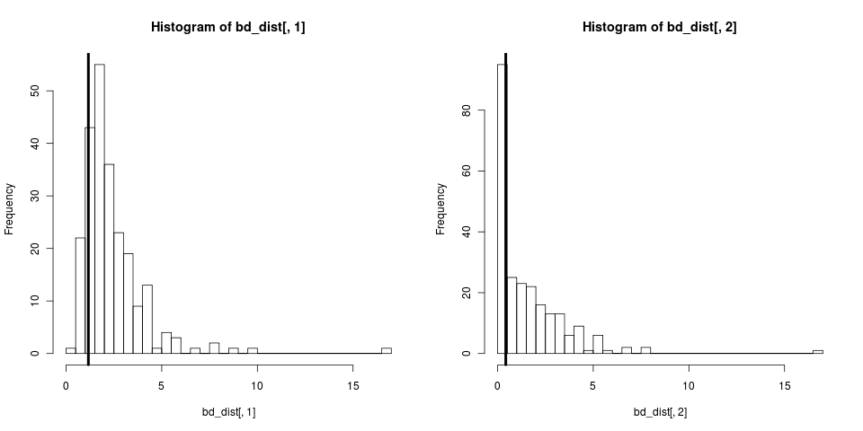
This didn’t condition on reality of N species being observed. We can repeat with sim.bd.taxa
  tree <- sim.bd.taxa(n=50,numbsim=1,lambda=2,mu=0.9,
                      complete=FALSE)[[1]][[1]]
  fit <- bd(branching.times(tree))
  para <- swp(fit$r, fit$a)
# simulate lots of trees
  boots <- sim.bd.taxa(n=50, numbsim=500, lambda=para[1], mu=para[2],
                      comp=FALSE)[[1]]
  bd_dist <- sapply(boots,
              function(x){
                fit <- try(bd(branching.times(x)))
  ## Some fits fail because bd sucks too.  tell R to tough it out anyhow
                if(!is(fit, "try-error"))
                  para <- swp(fit$r, fit$a)
                else
                  para <- NA
                c(para[1], para[2])
              })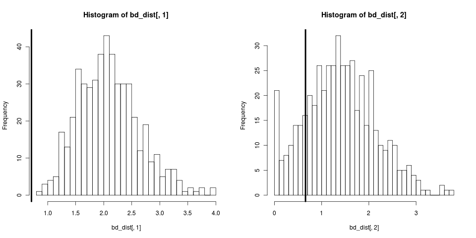
How about David’s question on bootstrapping the likelihood? How about when the birth-death model is inappropriate to the data? Here we will tranform the tree to create a topology very different than any we’ve seen, where branching starts off rapidly and then seems to stop:
Birth-death trees are quite twiggy, this seems like a rather unlikely tree for a birth-death process. 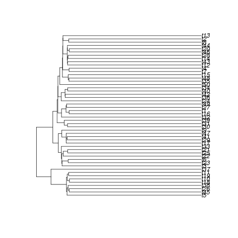
  tree <- sim.bd.taxa(n=50,numbsim=1,lambda=2,mu=0.9,
                      complete=FALSE)[[1]][[1]]

  tree <- lambdaTree(tree, .2) ## TRANSFORM THE TREE
  fit <- bd(branching.times(tree))
  para <- swp(fit$r, fit$a)
# simulate lots of trees
  boots <- sim.bd.taxa(n=50, numbsim=500, lambda=para[1], mu=para[2],
                      comp=FALSE)[[1]]
  bd_dist <- sapply(boots,
              function(x){
                fit <- try(bd(branching.times(x)))
  ## Some fits fail because bd sucks too.  tell R to tough it out anyhow
                if(!is(fit, "try-error")){
                  para <- swp(fit$r, fit$a)
                  lh <- fit$LH
                }
                else {
                  para <- NA
                  lh <- NA
                }
                c(para[1], para[2], lh)
              })
  bd_dist <- t(bd_dist)

  ## give us a wee peek at some summary data
  print(summary(bd_dist))
  print(sd(bd_dist, na.rm=T))

  png("bddist.png", width=480*3)
  par(mfrow=c(1,3))
    hist(bd_dist[,1], breaks=30, main="b")
    abline(v=fit$r, lwd=4)
    hist(bd_dist[,2], breaks=30, main="d")
    abline(v=fit$a, lwd=4)
    hist(bd_dist[,3], breaks=30, main="lik")
    abline(v=fit$LH, lwd=4)
  dev.off()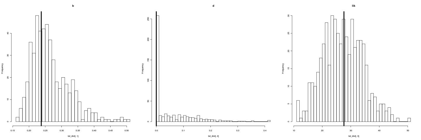
However, the bootstrap of likelihood (rightmost histogram) does not register as such a bad fit. Testing model adequacy requires a richer approach. The bootstrapping estimates our uncertainty under the assumption that our model is reasonable.
A footnote on strange behavior in TreeSim
Some computers (my laptop) geiger’s prune.extinct.taxa or Tanja’s option to return a only extant taxa (complete=FALSE) end up dropping all tips always. This bug (after some effort and help from mailing lists yesterday) is caused by having: Sys.setlocale(locale=“en_US.UTF-8”) and can be fixed by using Sys.setlocale(locale=“C”) see mailing list threads…
References
- Stadler T (2011). “Simulating Trees With A Fixed Number of Extant Species.” Systematic Biology, 60. ISSN 1063-5157, https://dx.doi.org/10.1093/sysbio/syr029.