Our little informal ABC group met again today to continue our discussion of ABC methods from last week. The updated code is included in the gist below. ((Nick asked about gists – they are code boxes provided by Github that are easy to embed into blogs, etc. They provide automatic syntax highlighting and version management. For instance, I just opened last week’s gist and started editing during today’s session – when I save it I get a new version ID, so last week’s post still points to last week’s code, but it doesn’t create a second copy, so you can tell if you have the right version. Click on the gist id at the bottom and you can see the revisions.))
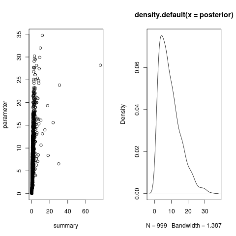
The posterior distribution from the regression
The regression is used to determine the posterior distribution of the parameter. We want to move each the observed values down along a line parallel to the regression line until they are at a point at the observed summary statistic. We do this as
\[\theta_i^* = \theta_i - b(S(X_i) - S(X_0)) \]
where b is the slope of the regression, S(X_i) is the summary stat on each of the simulated data in the regression, and $ S(X_0) $ is the summary statistic of the observed data. The distribution of these $ _i^* $ is the posterior distribution of theta. (see Figure 1 of (Csilléry et. al. 2010)).
[gist id=914487]
Comparing models
We consider the alternative model that the data comes from the gamma distribution, rather than the normal distribution, in the example above. We’d like to compare the models by Bayes factors. ((We are just using the single summary statistic, the mean, in both cases. This should be a sufficient statistic to estimate the mean of the normal, the mean of the gamma model is the product of the rate parameter and the shape parameter.))
The Bayes Factor is the ratio of the probability of the data under model 1 vs the probability of the data under model 2, which we get by integrating out (marginalizing over) the possible parameter values of the model:
\[\frac{P(X|M_1)}{P(X|M_2)} = \frac{ \int P(X|\theta_1) P(\theta_1) d\theta_1 }{ \int P(X|\theta_2) P(\theta_2) d\theta_2} \]
We don’t know the likelihood, $ P(X | _1) $, etc, but argued that by Bayes Theorem we could replace it with the posterior we just calculated, using $ P(X | _1) P(_1)$ with $ P(_1 | X)P(X)$. Then P(X) cancels out of top and bottom, and we’re left with
\[\frac{P(X|M_1)}{P(X|M_2)} = \frac{ \int P(\theta_1 | X) d\theta_1 }{ \int P(\theta_2 | X) d\theta_2} \]
Is this correct? What should these integrals be normalized by? Guess we better check our references.
CORRECTION: (2 May 2011)
P(X) is model dependent, lost in my sloppy notation. Rather than showing all models are equal (ratio of integral of posteriors above is unity) we have
\[\frac{P(X|M_1)}{P(X|M_2)} = \frac{ \int P(\theta_1 | X)P(X|M_1) d\theta_1 }{ \int P(\theta_2 | X) P(X|M_2) d\theta_2} \]
Which is simply not useful, as it recovers our original expression (Factor out the P(X) terms and the posteriors just integrate away. Instead, we are just left with the regular integrals to compute, probably by MCMC. Knowing the posterior distributions doesn’t seem to help in the computation of the Bayes Factors. Worth seeing other work on computation of Bayes factors, such as why we end up with Harmonic means, stepping stone approach, etc etc.
Next time
Verify/finish the model comparison between normal and gamma
Multi-parameter inference
Family-of-models comparisons?
Maybe take a look at efficiency improvements such as in (Wegmann et. al. 2009)
Get ready for our next algorithm (MCMC, HMM, EM). We discussed ABC-MCMC, so might want to consider (Marjoram, 2003) and its criticisms in (Wegmann et. al. 2009). Re HMM, again may be natural to build from the ABC, see C. Robert’s post, and a recent paper on the arxiv.
Try implementing automatic estimates for summary statistics? see paper, via C. Robert’s blog.
References
Csilléry K, Blum M, Gaggiotti O and François O (2010). “Approximate Bayesian Computation (Abc) in Practice.” Trends in Ecology & Evolution, 25. ISSN 01695347, https://dx.doi.org/10.1016/j.tree.2010.04.001.
Wegmann D, Leuenberger C and Excoffier L (2009). “Efficient Approximate Bayesian Computation Coupled With Markov Chain Monte Carlo Without Likelihood.” Genetics, 182. ISSN 0016-6731, https://dx.doi.org/10.1534/genetics.109.102509.
Marjoram P (2003). “Markov Chain Monte Carlo Without Likelihoods.” Proceedings of The National Academy of Sciences, 100. ISSN 0027-8424, https://dx.doi.org/10.1073/pnas.0306899100.