Lab Notebook

Working on my SICB talk, going a little further into the example of fitting the lambda model on the Anoles data to illustrate the ways in which we may lack sufficient data for the question.

1. The dataset may not contain adequate signal of the parameter / phenomenon in question

2. The dataset may not be adequately large

Anoles data set (23 taxa):

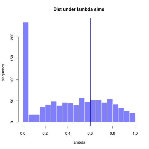
This first image shows the distribution of lambda values estimated from many datasets all simulated under a lambda = 0.6.  (Replotted from earlier entry)

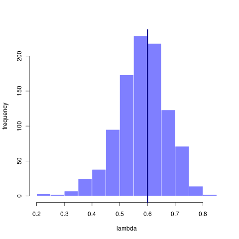
A larger (simulated > 300 taxa) tree has can infer lambda with somewhat greater accuracy, though still rather sizable variance. (reran this simulation from earlier entry code that didn’t store the .Rdat file)

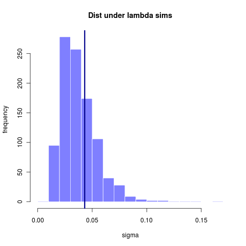
How informative the data are depends on the question.  Using the original 23 taxa tree we find it is plenty big enough to reliably recover the estimate of sigma, even though many of those estimates come from models that have rather mismatched lambda.  This suggests that sigma is nearly a sufficient statistic, while lambda is not.  That it can fit even when lambda is mismatched further suggests that the tree itself isn’t informing that estimate much – simply matching the variance in the data is most important.  This apparent lack of phylogenetic signal, however, says everything about how small the tree is, not how well or not well Brownian motion fits the data.

My last post was a bit pessimistic, sometimes I can still miss the forest for the trees.  Hidden in those figures, the main point has been staring me in the face.  So let’s try this again.

Stochastic limits to evolutionary branching is the story of two dueling timescales.  The first timescale is that of the evolutionary process: the frequency of steps (mutation rate, $ $) and the size of the steps (mutation kernel standard deviation $ _{}$), on top of which we add the selection gradient, created by the ecology. The second timescale is that of ecological coexistence, which in low noise situations should be much longer, and hence irrelevant.

While the approach to the branching point depends on the width of the resource kernel and is independent of the competition kernel.  At the branching point, how much narrower the competition kernel is compared to the resource kernel (in units of the mutational step size) determines how stable the coexistence of the early dimorphism is – the second timescale.  In most adaptive dynamics simulations this second timescale is irrelevant, being much longer than the former timescale, at least by assumption.  However, this need not be the case.

When this timescale (influenced by most parameters: population size, mutation size relative to competition kernel; resource kernel matters more weakly[ref] should add the equations for approximating the coexistence time to illustrate this[/ref])  becomes on the same order as the evolutionary timescale of waiting until the next mutation (determined by the mutation rate and population size) suddenly it impacts the waiting time until branching.

This can be characterized by the number of times a dimorphism establishes but then fails.  Similarly, weak coexistence impacts the number of times the dimorphism survives long enough for the mutation to arrive and establish, only to again collapse.

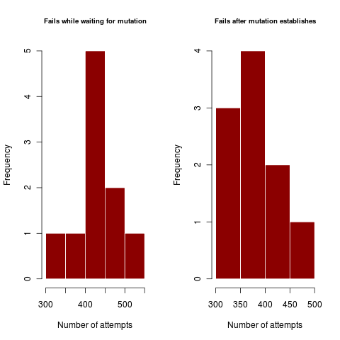
Figures illustrate outside the regime where coexistence times matter, where dimorphism never collapses after establishing.  In harsher parameter regime, the dimorphism collapses hundreds of times before enough mutations can accumulate in rapid succession (or a rare large mutation occurs) to create a dimorphism of substantially different traits so as to coexist.

Respective codes for each figure to show parameter values:

 all[[2]] <- ensemble_sim(rep=rep, sigma_mu = 0.05, mu = 1e-3, sigma_c2 = .1, sigma_k2 = 1, ko = 500, xo = 0.1, threshold = 30)
 all[[3]] <- ensemble_sim(rep=rep, sigma_mu = 0.03, mu = 5e-4, sigma_c2 = .3, sigma_k2 = 1, ko = 500, xo = 0.1, threshold = 30)

(full code).

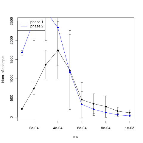
In the first example, a mutation at least two standard deviations out (prob <5%) from the expected value is sufficient to get a standard deviation away from the competition kernel (i.e.  60% competition).  Step-size limited mutations should have very similar failures for the first and second plots, using lots of little steps each with high failure rate.  Mutation-rate limited processes use one big jump, and show a high disparity between the failures in the first case and failures in the second.

Figures like the above show that when coexistence is hard (sigma_c  approaches sigma_k = 1) failure rates can be very high.  As the rates are very similar, this case appears to be clearly step-size limited, proceeding through many mutations with low probability of success of coexisting.

(code & data)

Further Exploration: Illustrating this second mode (mutation-limited)

Trying some examples now to see if I can create mutation-rate limited example by running the above at sigma_mu=.5 rather than .3 when varying mutation rate over 1e-4 to 1e-3.

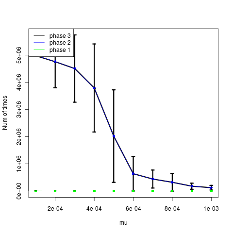
The low mutation rates appear to time out instead (time until phase, left figure).  The higher mutations actually show slightly fewer attempts after establishment, but not a strong signal.  Trying now with larger mutation steps.

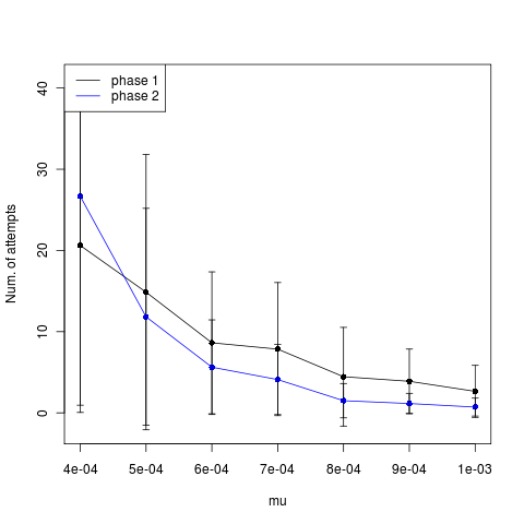
Still shows no indication of rate limited mutation.

In addition to my primary research categories, I make some entries in my lab notebook  to document and reflect on my experiment in open notebook science.  This includes my notes on tools I try out for open and collaborative science, including uses of social media, cloud computing, and scientific databases and repositories.

This serves as a cover-page for the open science entries in my notebook, displaying the most recent entries, articles, figures and code through rss feeds.

Recent Notebook Entries

[rssinpage rssfeed=‘https://www.carlboettiger.info/archives/category/ons-thoughts/feed’ rssformat=‘x: Y’ rssitems=“10” rssdateformat=‘j F Y’ rsstimezone=‘America/Los_Angeles’]

Entries from before 20-Oct-2010

Recently Added Articles

I maintain a collection of literature on articles that discuss the future of science, peer review, open access, open data, web tools and science 2.0 ideas on Mendeley called “Future of Science,” whose rss feed appears below.

[rssinpage rssfeed=‘https://www.mendeley.com/groups/530031/future-of-science/feed/rss’ rssformat=‘x: Y’ rssitems=“5” rssdateformat=‘j F Y’ rsstimezone=‘America/Los_Angeles’]

Recent Figures

[flickr-gallery mode=“tag” tags=“ons” tag_mode="all"]

Code Updates

I’m developing an R package called “socialR”, which I use to interact with my notebook, github code library, flickr image database and twitter  notification system from within R.  These are the updates from the commit log, see this entryfor details.

[cetsEmbedRSS id=https://github.com/cboettig/socialR/commits/master.atom itemcount=5 itemauthor=0 itemdate=1 itemcontent=0]

Ran a series of simulations overnight to explore aspects of time-to-branching at different phases of the branching process.  Still using only 16 replicates per data point, though increased maximum time for a run another order of magnitude to avoid timing out runs influencing the dataset for the slow-rate parameters.  Still seems to suggest a regime beyond which branching becomes completely improbable.  Not clear that the transition is a sharp as the Arrhenius approximation might suggest.

[flickr-gallery mode=“tag” tags=“2010dec30slideshow”]

(code)

(data)

[flickr-gallery mode=“tag” tags=“adaptivedynamics”]

I have found the interpretation of the larger scale simulations exploring the impact of the various parameters upon the branching times in different phases somewhat less clear than I had hoped.

The analytical approximation gives the suggestion of a sharp transition between a regime where branching is “easy”, where the expected coexistence times are longer than the expected waiting time to the next mutation, and “hard”, where they are shorter. The mathematics reduce to an expression similar to the Arrhenius law, where there is a sharp transition between the probability of being in one state to being in the other depending on the noise level.

I have been trying to get explore this through the simulations and figuring out the best way to visually represent this. I have been using the contour plots you suggested to illustrate the coexistence times on the PIP, which is quite nice. Unfortunately the analytic approximations don’t seem to agree quantitatively outside a somewhat limited parameter range, more limited than I expected.

I have also been exploring the time required to reach each of our four phases of the branching process as a function of the various parameters. In this I hoped to see the sharp transition predicted by the approximation, but figuring out the best way to both explore and visualize this through the parameter space. Hard to distinguish this from simply getting exponentially longer.

Setting up some adaptive dynamics simulations to complete the parameter-space search.  Currently the demo library contains two files, providing the coexistence-only tests and the full evolutionary simulation.  This picks up from Aug 30/Sept 1 on coexistence times and Aug 12/13 entrieson waiting times until branching (while still on OWW).

coexistence times

coexist_times.R creates contour plots of the coexistence time under demographic noise expected at a particular position of the pairwise invasibility plot (PIP).  I also attempt to calculate these using an analytic approximation derived through the Arrhenius law trick to the SDE approximation.

ensemble_coexistence() runs just the coexistence simulation from

coexist_analytics() attempts to create the same graph analytically.

Unfortunately the analytic approximation seems insufficient:

[flickr-gallery mode =“tag” tags=“contour_analytics_vs_simulation”]

Phases of the branching Process

ensemble_sim() runs the full simulation with mutations.  Returns an ad_ensemble object with three elements: $data, $pars, and $reps.  $data is a list element for each replicate.  For each replicate, it records 4 time-points:

1. First time two coexisting branches are established

2. Last (most recent) time two coexisting branches were established

3. Time to finish phase 2: (satisfies invade_pair() test: trimorphic, third type can coexist (positive invasion), is above threshold and two coexisting types already stored in pair

4. Time to Finish line (a threshold separation): traits separated by more than critical threshold

For each of these it returns the trait values of the identified coexisting dimorphism as well (x,y).  This x,y data is plotted for all replicates in four butterfly plots (for each time interval) by plot_butterfly.  Time data is coded in the shading. (just call plot_butterfly on the ad_ensemble object).

In addition to these four (t, x, y) triplets, each replicate reports two counts:

1. Number of times the dimporphism is lost in phase 2

2. Number of times the dimorphism is lost in phase 1

These are histogrammed by plot_failures(object).  Finally, plot_waitingtimes(object) just histograms the distribution of waiting times  across replicates for each of the four phases outlined above.  Figures from today’s version of waiting_times.R

[flickr-gallery mode=“tag” tags=“waiting_times”]

Illustrating Key Phenomena

The motivation for these two lines of investigation go back to simulations from May 3-4 entries which begin to show distinction between different mechanisms of branching.  The hint comes between processes that appear limited by phase 1 an those limited by phase 2.  This can be illustrated by the time required or the number of attempts necessary (failure rate histograms).

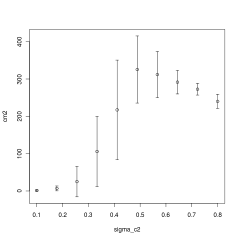
Running simulation sets now varying the range of sigma_mu, sigma_c2, and mu to illustrate the sharpness of the transitions between noise-limited and not limited branching dynamics, and how the difference in times and attempts between phases changes with these parameters.  i.e.

Computing Notes:

Setup AdaptiveDynamics repository on zero.  An outdated rsa_id key in /.ssh was causing me not to be able to commit from

This time of year I have to file my renewal for my DOE Fellowship, including a statement of accomplishments and a summary of the computational aspects of my work.  Seemed like a good idea to jot these down in my notebook as well:

synopsis of accomplishments over the year:

In January I passed my qualifying exam, advancing to candidacy where my dissertation remains my only requirement.  In March I attended the phylogenetics workshop in Bodega Bay, an internationally known week-long training program.  I also attended the CSGF conference in June, and gave talks at both the Evolution conference and the integrative phylogenetics conference, iEvoBio, in July, both key events in my field.

From the beginning of June until the start of September, I stepped outside my research in phylogenetic models to focus on stochastic population dynamics.  While the details of this project are described in my practicum evaluation, the mathematical and computational tools I learned in the process have found surprisingly apt applications in my phylogenetics research, where they have helped me solve a key problem in my thesis.  Since this breakthrough, I have been focused on writing up two manuscripts which have been made possible by this step forward.

As my computational needs surpass what is readily available through my lab servers, I have learned to leverage Amazon’s cloud computing for rapid deployment of large-scale simulations and analyses. Overall, this has been a productive year, translating what I’ve learned in my POS classes into practical research experience and making some important steps in my thesis.  I look forward to the next year of synthesizing and writing up these results and continuing to build on the methods and tools I’ve learned and developed.

describe concisely what you regard as the most interesting and innovative aspects of your current research, with special emphasis on computational science.

My research combines the recent explosion of data available through gene sequencing and subsequent readily available phylogenetic information with the power of high-performance computational approaches to “replay the tape” of evolution to better understand the origins and maintenance of biodiversity.

Genetic data paved the way to phylogenetic inference, the mapping of ancestor-descendant relationships between the species living today.  These phylogenies become my periscope into the past.  In the absence of fossils, I can simulate different evolutionary models of selection on various traits retracing the phylogenetic tree to discover which models are most consistent with the patterns in species we observe today. By running the stochastic simulation repeatedly, I can create not only one possible outcome, but the parameter space of all possible outcomes and their associated probabilities.  This planet has run the experiment of evolution only once, but using this computationally intensive approach I can run that process over and over again under different assumptions, allowing me to explore evolutionary questions that can be answered no other way.

My own reflections and list

Hmm, the research summary with computational emphasis is kinda vague, but aiming for a non-specialist audience.  Hard to differentiate between the aspects that really leverage HPC and those that can be adequately run at the desktop level.  Is that really the best statement of my accomplishments?  I might try a different format for myself:

• Formulated and explored implications of my phylogenetic Monte Carlo approach.  Formulated throughout the Spring quarter, been writing and rewriting the manuscript most of this past Fall.

• Derived and implemented the heterogeneous alpha/sigma model (in a few busy days and a long train ride in July, waiting to write up after PMC is done)

• Used said model and phylogenetic Monte Carlo to demonstrate clear release-of-constraint in the Labrid data

• Exploring better early warning signal models and detection methods.  Settled on linearized models of the canonical form of two bifurcation types, identifying warning signals directly by a similar Monte Carlo test to the phylogenetics example.

• Explored stochastic population dynamics in structured populations via the ELPA tribolium model.  Negative feedbacks mean no large-amplification demographic noise, but cycles do break down the linear noise approximation.  (a few weeks in May and June)

• Rebuilt the Adaptive Dynamics code to illustrate how time to branching and coexistence times vary in parameter space (auto-generation of the butterfly plots, mostly two weeks in April)

• Began my open lab notebook (starting in January on OWW, migrated to Wordpress in Sept), public code hosting (initially google code, moved to github in March), Mendeley database (Oct ’09), Flickr only this Oct, and social media for science (Twitter only since July, though have used FF since the beginning of the year).

• Started AWS/cloud computing.  Still coding in C but using R more, parallelization in R’s snowfall.

In this spirit, Mendeley provides some easy data on what I’ve been reading:

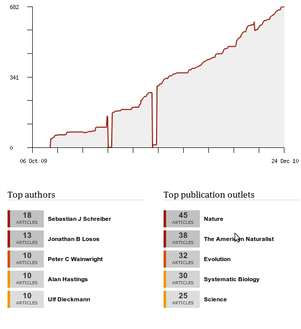
Interesting if not too surprising that my most popular authors are all advisors of mine, except Losos.  (Also it’s really obvious where I twice deleted my Mendeley database and needed their help support to recover my data… in only a few days).

.

Working on a few things in today’s lab notebook entry.  Some more notes on exploring cloud computing tools, sketching out some ideas for my #scio11 science online panel discussion on open notebook science, and otherwise working on my phylogenetics mansucript.

Cloud Computing

An interesting package was announced over the r-sig-hpc list today, creating an arbitrarily large Hadoop cluster out of Amazon EC2 instances directly from the R command line. JD Long has been very responsive to my naive questions on setting it up, so I was able to quickly activate an Elastic Map Reduce account via Amazon Web Services and run the example code. It installs an instance of R on each cluster at the time of launch, so it takes a moment to initialize and I’m not sure if it can handle calls in the parallel code that call other libraries (unless perhaps these are explicitly loaded in the parallel function?) The code essentially provides a parallel (elastic map reduce) version of lapply, running the instances on different machines (EC2 instances) and then sewing the answers back together.

As the interface is delightfully simple, could possibly be useful even to run single amazon instances. Simply set credentials, initialize a cluster of specified size and instance type, and then call the parallel lapply:

setCredentials("yourKey", "yourSecretKey", setEnvironmentVariables=TRUE)
myCluster <- createCluster(numInstances=5)
emrlapply(...)

Look forward to learning more about the package, EMR, and testing it out. Code available through Google code hosting.

Science Online 2011

Getting ready for Science Online Conference. Finalizing room share with Mark Hahnel and touching base with Jean-Claude Bradley and Tony Williams about our panel on Open Notebook Science. Jean-Claude describes that we’ll have a short introduction before launching into the panel discussion. His introduction will focus on how and why they can convert ONS data to web services (like ChemSpider, which Tony represents). Provide a nice parallel to what I’m trying to do integrating this notebook into web services. Using this notebook space to brainstorm a bit what I can contribute/would like to cover in the session.

Think my intro will try to highlight these three things:

• Open Notebook Science for Theorists

As theorists, it should be easier for us to keep electronic lab notebooks than for empiricists. We can blithely ignore all those discussions about having a laptops or ipads to write at the bench or gloves-on or gloves-off keyboards. We have a machine within easy reach. Most of the computational work is done on the computer already, where software solutions can track progress and changes automatically. and yet… it isn’t.

Perhaps the primary problem is that we’re not taught to keep lab notebooks in the first place. It might help if students in the sciences were taught software development practices like version managing, but we’re not. Capturing the abstract parts of theory is even harder. I don’t really know what the workflow of other theorists in my field looks like, even for people I work with closely. I guess that’s part of my desire to create an open notebook.

• Open Notebook Science from the perspective of a student

I started practicing open notebook science as a third year graduate student without input for or against the idea from my advisor or anyone else at my institution. I suppose there are a variety of stages or positions from which someone might first start an open lab notebook, and a variety of ways to do it. Each face a rather different set of challenges, and perhaps I can offer something of the student perspective.

• Integration of web services relevant to theory and computing

Integrating databases such as flickr/github/mendeley, now also Amazon web services; hopefully the databases like dryad eventually.  I’m interested to learn about the more mature models of integrating with external databases and how to make the most of this.

• The social dimension

I’ve described my efforts as a “social lab notebook.” That’s a little ambitious for something that no one else reads, let alone comments. But it’s a design principle of sorts.  I’m interested in how to do this effectively, and what potential it has to make better, faster, and farther reaching science.

Writing

Also continuing my phylogenetics writing today, working on explaining the models.  (current version of manuscript .tex file in github Phylogenetics repository).

Not really working today, as holidays approach, but came across the Gource toolkit for creating video visualization from git development (inspired by the Mendeley’s example). So in the spirit of year-in-review reflections, here’s my development from the past year (just for the phylogenetic statistics work).

Quality is a little too poor to read file names, more entertaining than practical. Other user icons appear in December corresponding with my move to running the code from Amazon cloud. The lower cluster includes the demos directory, the upper the R code, so gives some indication of extensions to methods vs testing applications. Captures my bursty code development, though perhaps not as well as the github graphs.

Notes for making the video

A couple steps. First just running gource (in ubuntu universe repositories) on the repository directory launches the video, used gtk-recordMyDesktop to capture the film (no luck with piping to ffmpeg). Then truncated, changed format, uploaded to youtube. Truncation and format conversion are simple bash commands:

# Shorten film 
 ffmpeg -sameq -ss 0 -t 900 -i testvideo.ogv gource.ogv
# convert to avi
 mencoder gource.ogv -nosound -ovc xvid -xvidencopts pass=1 -o gource.avi

Phylogenetics writing still continues.

AIC Error rates

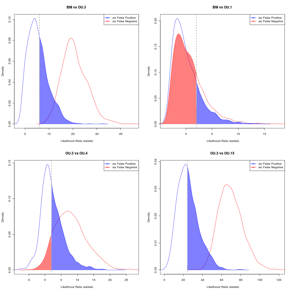
Choosing by  having < 5% probability of rejecting the simpler model when it is true.

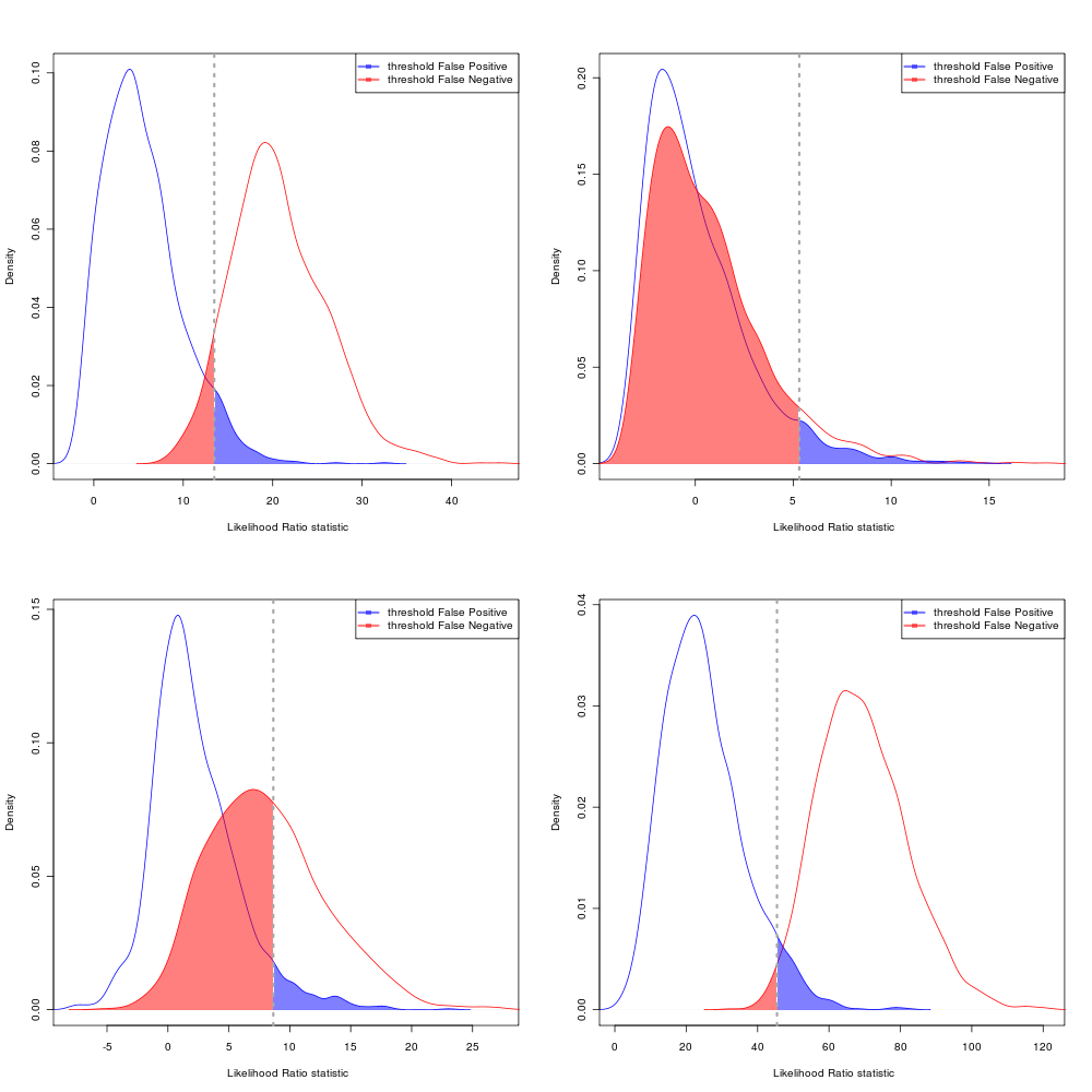
Choosing the equal-likelihood division: