### Power in Trees tests (Results from single OU simulation per alpha, run yesterday)
2000 replicates gives a cleaner picture of the critical alpha, though with low alpha values the estimates of p are quite variable. Also more variable on the smaller trees. Even arbitrarily large alpha aren’t significant on the 5-taxa primate tree. On the small geospiza tree (13 taxa) from the geiger package we find:
0.5735   0.29  0.704 0.6465  0.993  0.838 0.8605 0.9355  0.782  0.845   0.93
 "0.1"  "0.2"  "0.3"  "0.4"  "0.5"  "0.6"  "0.7"  "0.8"  "0.9"    "1"    "2"
 0.945 0.9985  0.958 0.7725 0.9995  0.982  0.949  0.992      1   0.99  0.999
   "3"    "4"    "5"    "6"    "7"    "8"    "9"   "10"   "20"   "30"   "40"
0.9895
  "50"
P values on top row, alpha values in quotes below the p value. Notice 9 fails to be significant at 0.95% confidence level, though might as easily be somewhere around 6. For the Labrid tree with 114 taxa the pattern is clearer though not perfect:
 0.621  0.502 0.9735   0.66 0.5185 0.8075 0.9975 0.9665  0.907  0.997 0.9945
 "0.1"  "0.2"  "0.3"  "0.4"  "0.5"  "0.6"  "0.7"  "0.8"  "0.9"    "1"    "2"
     1      1      1      1      1      1      1      1      1      1      1
   "3"    "4"    "5"    "6"    "7"    "8"    "9"   "10"   "20"   "30"   "40"
     1
  "50"
Significance clearly sets in between alpha of 0.9 and 1.
Summary:
> birds$min_alpha
[1] 10
13 taxa
> primates$min_alpha
[1] 1000
(5 taxa)
> carnivora$min_alpha
[1] 1
260 taxa
> labrids$min_alpha
[1] 1
114 taxa
> carex$min_alpha
[1] 2
53 taxa
>
reducing the noise in the power estimation
I’ve just implemented the power test for the smallest alpha that can be detected at the 95% level using the (whatarewecallingitnow) likelihood ratio monte carlo approach on a given tree. I try simulating under successively higher alpha values and then see if the resulting dataset can be distinguished. In my first implementation, this involves only one simulation from the OU model at a given alpha, and then the N bootstrap simulations from the null brownian model per alpha.
Obviously I want more than one simulation from the OU process. It seems I could (1) simulate under the OU model of a given alpha, (2) fit the BM model to the resulting data, (3) simulate under that BM model to get the “bootstrap” data, for which (4) I refit the BM and OU models and compare the likelihood ratio of these refit models. That sounds pretty convoluted when I describe it that way, but I think this is the “natural” thing to do? i.e. steps 2-4 are the bootstrap process which I normally repeat N times for a single dataset, now instead of using a single dataset I draw a dataset from the distribution….
New approach: multiple simulations from alpha ———————————————
Plots show decreasing power with decreasing alpha
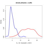

Anoles data at alpha=25. Red curve is the LR distribution when simulations come from OU with alpha=25, blue line is LR distribution when simulations come from BM models fit to those OU-generated data
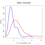
Anoles data at alpha=1.
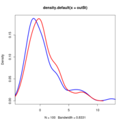
Anoles data at alpha=0.25.
New procedure:
   ## Draw a data sample from the distribution produced by test
    data <- simulate(test, n=nboot)

    ## fit the null models to these data -- so we simulate from the appropriate null
    nulls <- lapply(1:nboot, function(i){
            update(null, data[[i]])
    })
    tests <- lapply(1:nboot, function(i){
            update(test, data[[i]])
    })
    t0_dist <- sapply(1:nboot, function(i){
        if(is(tests[[i]], "hansentree")){ t0 <- -2*(nulls[[i]]@loglik - tests[[i]]@loglik) }
        else { t0 <- -2*(nulls[[i]]@loglik - tests[[i]]$loglik) }
    })


    ## Data come from a distribution of nulls,
    X <- sapply(1:nboot, function(i){
        simulate(nulls[[i]])
    })

    t <- sapply(1:nboot, function(i){
        refit_null <- update(null, X[[i]])
        refit_test <- update(test, X[[i]])
        if(is(refit_test, "hansentree")){ out <- -2*(refit_null@loglik - refit_test@loglik) }
        else { out <- -2*(refit_null@loglik - refit_test$loglik) }
        out
    })

 plot(density(out$t), col='blue', lwd=3,xlim=range(c(out$t0_dist,out$t)) )
 lines(density(out$t0_dist), col='red', lwd=3)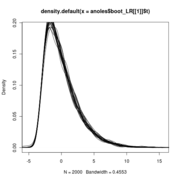
Null distributions of the LR all lie on top of eachother regardless of sigma
From these it is possible to estimate the power (see powertest.R code)
Note that the null distribution (the blue curve) doesn’t actually differ and so doesn’t need to be re-simulated with different values.
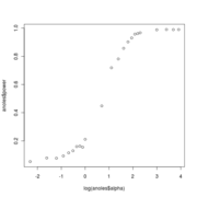
anoles power
Meanwhile ———
- Finishing the story on model choice in the Anoles dataset. Resimulating with extra replicates and including all 5 original models.
- Good news is that 2000 bootstraps on all 6 models against each other is quite fast on the 16-processor zero, an hour or so. Bad news is the ou2 funny painted model isn’t bootstrapping the LR correctly, though all the other pairs are.
- Other sorta bad news is that OU_LP does a handy job at beating all other models under Monte Carlo Likelihood Ratio test, so the final conclusion doesn’t have the punchiness a contradiction would. At least the contrived OU2 contradicts this. Should also add the “all different” painting to the mix to demonstrate. –Carl Boettiger 01:24, 27 August 2010 (EDT) Fixed, order of nodes conflicted.
Slideshow of results
![]()
![]()
Code updates
–Carl Boettiger 03:26, 27 August 2010 (EDT)
Just implemented the fast version of the power test, which avoids re-simulating from the Brownian motion null, and handles the parallelization with more finesse, and as a single function. Set to run examples overnight.
Removed the traitmodels support from the power test for the moment, until the convergence issues are dealt with. The s3/s4 class differences to access elements make this annoying as method dependency must be handled explicitly by if statements not automatically by class generics. (guess could access by index? – Nope, S4 classes aren’t subsettable)
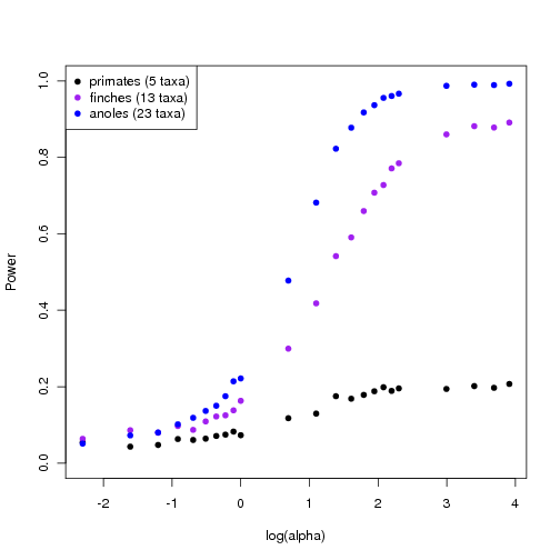
Updated power curves for trees
Using the faster approach avoiding re-sampling the null distribution for each alpha, I generate power curves for trees of different sizes and complexity. The larger, richer trees show more power.