editorial note: These notes pre-date the formal start of my online laboratory notebook, Feb 2 2010: The Lab Notebook Goes Open and were adapted from a LaTeX document in which I kept notes on this topic during my summer at IIASA. Lacking a proper notebook then, documents like this one were updated periodically and occassionally branched into new ones. The post date represents the last time the LaTeX document was edited in the course of that research.

Extinction Probabilities

Gardiner (1985).

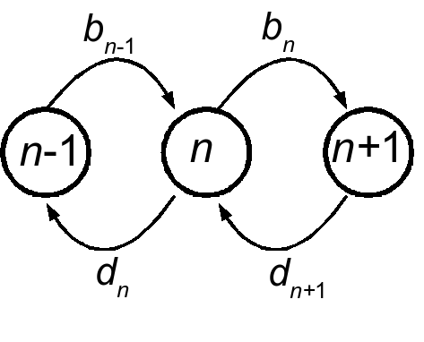
We consider single-step birth death models for the majority of this work. Though they will become multidimensional in later parts of the work, as we deal with multiple species or explicit environmental changes, for the time being we will focus on the one-dimensional bith-death process. The Markov process is defined over positive integers, \(n \in \mathbb{Z}^+\), and will sometimes be assumed to be bounded above by some integer \(N\). The process is determined by two state-dependent rates, \(b(n)\) and \(d(n)\), as depicted here:

The process is specified by the Master equation:

\[\frac{\partial P(n,t)}{\partial t} = b(n-1)P(n-1,t)+d(n+1)P(n+1) - \left( b(n) + d(n) \right) P(n) \label{mastereq}\]

and approximated by the method of Kurtz (1971) or van Kampen’s linear nois expansion as:

\[\frac{\partial P(\tilde n,t)}{\partial t} = - \underbrace{\frac{\partial \left( b(\tilde n)-d(\tilde n) \right)}{\partial \tilde n}}_{A(\tilde n) } \frac{\partial}{\partial \tilde n} \tilde n P(\tilde n,t)+ \underbrace{\frac{b(\tilde n)+ d(\tilde n)}{2} }_{B(\tilde n)/2} \frac{\partial^2}{\partial \tilde n^2} P(\tilde n) \label{forward}\]

Note that \(n\to \tilde n\) where \(\tilde n \in \mathbb{R}\) has become a continuous value in the limit of large system size. The coefficients \(A(x)\) and \(B(x)\) are the jump moments \(\partial_x \alpha_{1,0}(x)\) and \(\alpha_{2,0}(x)\) in the van Kampen expansion. This expression is known as the forward Kolmogrov equation. Its solution is a Guassian, with mean and variance given respectively by

\[\begin{aligned} \frac{\mathrm{d}x }{\mathrm{d}t} &= b(x)-d(x) \nonumber \\ \frac{\mathrm{d}\sigma^2}{\mathrm{d}t} &= A(x) \sigma^2 + B(x) \label{moments}\end{aligned}\]

Related to  is the backward Kolmogrov equation which we use for first-passage time problems:

\[\frac{\partial P(\tilde n,t)}{\partial t} = A(\tilde n) \frac{\partial}{\partial \tilde n} P(\tilde n,t)+ \tfrac{1}{2} B(\tilde n)\frac{\partial^2}{\partial \tilde n^2} P(\tilde n) \label{backward}\]

From this we have the first passage time starting at \(x\) across an absorbing boundary \(a < b\) given \(b\) is reflecting:

\[T(x) = 2 \int^x_a \frac{\mathrm{d}y}{\psi(y)} \int_y^b \frac{\psi(z) }{B(z)} \mathrm{d}z \label{firstpassage}\]

where we define the integrating factor

\[\exp\left( \int_a^y \mathrm{d}x \left[ \frac{2 A(x)}{B(x)} \right] \right) \label{integrating factor}\]

It is useful to work these results out for some familiar models.

Levins Model

We first consider the Levins model:

\[\begin{aligned} b(n) &= c n \left( 1 - n/K \right) \nonumber \\ d(n) &= e n \label{levins}\end{aligned}\]

\(K\) is the number of patches, and also the convenient measure of system size. In the limit of large \(K\), \(\tilde n = \tfrac{n}{K}\) represents the fraction of occupied patches, and we have the coeffients:

\[\begin{aligned} & A(\tilde n) = c(1-2 \tilde n)-e \\ & B(\tilde n) = c \tilde n (1 - \tilde n) + e \tilde n\end{aligned}\]

By way of  we have the equilibrium mean and variance:

\[\begin{aligned} & \langle \tilde n \rangle = 1-\frac{e}{c} \\ & \langle (\tilde n - \langle \tilde n \rangle )^2 \rangle = \frac{e}{c}\end{aligned}\]

Logistic Model

A closely related model is the logistic with the following interpretation:

\[\begin{aligned} & b(n) = r n \\ & d(n) = \frac{r n^2}{K}\end{aligned}\]

Which has mean and variance both equal to \(K\), and coefficents:

\[\begin{aligned} & A(x) = r - \frac{2 r x}{K} \\ & B(x) = rx + \frac{rx^2}{K}\end{aligned}\]

editorial note: These notes pre-date the formal start of my online laboratory notebook, Feb 2 2010: The Lab Notebook Goes Open and were adapted from a LaTeX document in which I kept notes on this topic during my summer at IIASA. Lacking a proper notebook then, documents like this one were updated periodically and occassionally branched into new ones. The post date represents the last time the LaTeX document was edited in the course of that research.

We wish to establish the fate of a population into which a rare mutant is introduced near a branching point. Far from the branching point, we had only one concern - will the mutant survive? Near the branching point, we now have two concerns - the fate of the mutant and the fate of the original resident. For branching to proceed, both must persist. The traditional framework of density-independent diffusion theory is insuffient to handle this case. We must consider both resident and mutant populations, with abundances \(N_1\) and \(N_2\) respectively. Under a series of approximations, we can again write this case as a one dimensional equation in the frequency of the mutant, \(p\); however, this time the equation will necessarily be nonlinear to have an additional intermediate stable state \(0<p<1\) in addition to the boundaries \(p=0\) and \(p=1\). We briefly review the necessary approximations as an understanding of them is essential to develop the proper picture.

While the argument could be expressed in greater generality of generic birth and death rates, working with our particular example is instructive. For a dimorphic population, the master equations governing the probability distributions are:

\[\begin{aligned} \frac{\mathrm{d}}{\mathrm{d}t} P(N_1,t) &= (\mathbb{E}_1 - 1) r N_1 \frac{N_1 + C(x_1, x_2) N_2}{K(x_1) }P(N_1) + (\mathbb{E}_1^{-1} - 1)r N_1 P(N_1) \nonumber \\ \frac{\mathrm{d}}{\mathrm{d}t} P(N_2,t) &= (\mathbb{E}_2 - 1) r N_2 \frac{N_2 + C(x_2, x_1) N_1}{K(x_2) }P(N_2) + (\mathbb{E}_2^{-1} - 1)r N_2 P(N_2), \label{mastereq}\end{aligned}\]

where \(E_i^k\) is the step operator taking \(f(N_i) \to f(N_{i+k})\). We apply van Kampen’s expansion of the master equation to linear order in the system size \(K_0\), the carrying capacity at the singular strategy. While several other options are possible, it is important to note that this approximation, which gives rise to a diffusion equation, is not based on the assumption of a large population size, but a large system size. Confusing the two is common in the literature. For instance, if the system size is an area, then the transformed variable that obeys the diffusion equation is the density of individuals (a naturally continuous quantity), not the number of individuals, and the approximation becomes better when larger areas are considered, not larger numbers in the same area (which just means a higher density). Having stated this, we take \(n_i = N_i/K_0\) and apply the expansion to recover the following stochastic differential equation (Itô expression)

\[\begin{aligned} \mathrm{d}n_1 = r n_1 \left(1 - \frac{n_1 + C(x_1, x_2) n_2}{K(x_1) } \right) \mathrm{d}t + \frac{1}{\sqrt{K_o} } \sqrt{r n_1 \left(1 + \frac{n_1 + C(x_1, x_2) n_2}{K(x_1) } \right) } \mathrm{d}W_1 \label{sde}\end{aligned}\]

and \(n_2\) similarly. This approximation is rigorously justified in the limit \(K_0 \to \infty\). The next approximation is only heuristically justified at the moment, changing variables into \(p = n_1/(n_1+n_2)\). The approximation makes two assumptions which are not strictly valid but justifable under the right conditions. The first is that the total population size is a constant, \(n_1 + n_2 = n\). Even at stationary state, this is not valid as the populations fluctuate according to , but these fluctuations become negligible for large \(K_0\). However, the system is only near stationary state when \(p\) is at it’s equilibrium value - it is not valid for all \(p\). This is more problematic, as the resulting SDE will depend only on \(k_1\) and not \(k_2\). Only when \(k_1 = k_2\) is this equation valid for any value of \(p\). If mutational steps are small this will be approximately true. As we will see, smaller mutational steps will require larger populations and/or tighter competition kernels for branching to occur at all. Simplying notation by \(C(x_1, x_2) = C_{1,2}\) and \(K(X_i) = k_i\), this gives us the one-dimensional nonlinear SDE in the frequency \(p\):

\[\begin{aligned} \mathrm{d}p = r p \left(1 - n \frac{p + c_{1,2}(1-p) }{k_1 } \right) \mathrm{d}t + \frac{1}{\sqrt{K_o n} } \sqrt{r p \left(1 + n\frac{p + c_{1,2} (1-p) }{k_1 } \right) } \mathrm{d}W_1\end{aligned}\]

The extinction probability \(u(p,t)\) for this expression is given by the Backwards equation for the generator,

\[\frac{\mathrm{d}}{\mathrm{d}t} u(p,t) = r p \left(1 - n \frac{p + c_{12}(1-p) }{k_1 } \right) \partial_p u(p,t) + \frac{1}{2K_o n } r p \left(1 + n\frac{p + c_{12} (1-p) }{k_1 } \right) \partial_p^2 u(p,t) \label{u}\]

with the boundary conditions \(u(0) = 1\) and \(u(1) = 1\) being absorbing.

After some rearrangement we can rewrite this as

\[\begin{gathered} \frac{\mathrm{d}}{\mathrm{d}t} u(p,t) = \left( rp \left( 1-\frac{n c_{12}}{k_1} \right) - \frac{r n}{k_1} p^2 (1 - c_{12} )\right) \partial_p u(p,t) \\ + \left( rp \left(1+\frac{n c_{12}}{k_1}\right) + \frac{r n }{k_1} p^2 (1 - c_{12} ) \right) \frac{\partial_p^2 u(p,t)}{2K_0 n}\end{gathered}\]

Note then for \(p\) small we can neglect the terms quadratic in \(p\) and we are left with the backwards equation from the density independent case,

\[\frac{\mathrm{d}}{\mathrm{d}t} u(p,t) = rp \left( 1-\frac{n c_{12}}{k_1} \right) \partial_p u(p,t) + rp \left(1+\frac{n c_{12}}{k_1}\right) \frac{\partial_p^2 u(p,t)}{2K_0 n}\]

Setting equal to zero we have a simple ordinary differential equation for the stationary extinction probability:

\[\begin{aligned} u &= 1 - e^{-2sp K_0 n} \\ s &= \frac{r\left( 1-\frac{n c_{12}}{k_1} \right) }{ r\left(1+\frac{n c_{12}}{k_1}\right)} \end{aligned}\]

and particularly for a frequency \(p\) corresponding to a single individual, a frequency of \(p=1/(N_1+N_2) =(1/K_0)/(n_1+n_2) = 1/(K_0 n)\), this reduces to

\[u = 1-e^{-2s}\]

Assuming $ rp ( 1- ) 0$, the time-dependent solution is:

\[\begin{aligned} u &= 1-e^{-p \psi(t) } \\ \psi(t) &= \frac{2 s K_0 n}{1-e^{ r\left( 1-\frac{n c_{12}}{k_1} \right) t } } \label{timedep}\end{aligned}\]

This tells us nothing about the survival of the resident. In most applications of this approach, it is assumed the resident quickly goes extinct once \(p \sim o(1)\). If we consider the asymptotic behavior of the nonlinear PDE, Eq. , we find not suprisingly that the asymptotic behavior is sure absorbtion at one boundary or the other. The asymptotic behavior needn’t concern us; as we really want to know how the expected lifetime of this dimporphic state compares with the rate at which mutants are entering this population. To do so we need the time dependent solution to the nonlinear equation .

This poses some trouble in choosing \(p = 1/(nK_0)\) as the initial mutant frequency. In the linear case, this always canceled perfectly with the noise term, \(nK_0\), leaving a fixation probability that did not depend on the population size (system size), given that it was large enough to justify the linear noise approximation in the first place. This is no longer the case. Larger populations result in the mutant frequency \(p\) being much smaller. While the noise also decreases, we do not observe the perfect balance of the linear system. While an analytic, time-dependent solution for \(u\) in this case is not possible, numerical solutions illustrate the much smaller populations having significantly higher survival probability, due to the higher value of \(p\) from which they start given a single mutation.

This seems unreasonable. A smaller population should be more suseptible to the accidental loss of a set of coexisting types, as observed in the simulations. I am unclear as to the explanation.

editorial note: These notes pre-date the formal start of my online laboratory notebook, Feb 2 2010: The Lab Notebook Goes Open and were adapted from a LaTeX document in which I kept notes on this topic during my summer at IIASA. Lacking a proper notebook then, documents like this one were updated periodically and occassionally branched into new ones. The post date represents the last time the LaTeX document was edited in the course of that research.

\[\begin{aligned} \mathrm{d}n_1 = r n_1 \left(1 - \frac{n_1 + C(x_1, x_2) n_2}{K(x_1) } \right) \mathrm{d}t + \frac{1}{\sqrt{K_o} } \sqrt{r n_1 \left(1 + \frac{n_1 + C(x_1, x_2) n_2}{K(x_1) } \right) } \mathrm{d}W_1\end{aligned}\]

\[\begin{aligned} p &= \frac{n_1}{n}, \quad q = 1-p = \frac{n_2}{n} \quad n = n_1 + n_2 \\ \mathrm{d}p &= \frac{\mathrm{d}n_1}{n}, \quad \mathrm{d}q = \frac{\mathrm{d}n_2}{n} \\ \mathrm{d}n &= \mathrm{d}n_1 + \mathrm{d}n_2 = n (\mathrm{d}p + \mathrm{d}q) \end{aligned}\]

\[\begin{aligned} \mathrm{d}p(p,n) = \alpha_1(p,n) \mathrm{d}t + \sqrt{ \alpha_2(p,n) } \mathrm{d}W_p \\ \mathrm{d}n(p,n) = \beta_1(p,n) \mathrm{d}t + \sqrt{ \beta_2(p,n) } \mathrm{d}W_n\end{aligned}\]

\[\begin{aligned} f_i(p) = r p \left(1 - n(p) \frac{p + c_{12}(1-p) }{k_i } \right) \\ g_i(p) = r p \left(1 + n(p) \frac{p + c_{12}(1-p) }{k_i } \right) \end{aligned}\]

\[\begin{aligned} \alpha_1 &= f_1(p) \\ \alpha_2 &= \frac{ g_1(p) }{K_0 n(p) } \\ \beta_1 &= n f_1(p) + n f_2(1-p) \\ \beta_2 &= n*\frac{g_1(p)+g_2(1-p)}{K_0 } \end{aligned}\]

\[\begin{aligned} \frac{\mathrm{d}}{\mathrm{d}t} \sigma_p &= 2 \partial_p \alpha_1(p,n) \sigma_p +2\partial_n\alpha_1(p,n) \langle p n \rangle + \alpha_2(p,n) \\ \frac{\mathrm{d}}{\mathrm{d}t} \sigma_n&= 2 \partial_n \beta_1(p,n) \sigma_n +2\partial_p\beta_1(p,n) \langle p n \rangle + \beta_2(p,n) \\ \frac{\mathrm{d}}{\mathrm{d}t} \langle p n \rangle &= \partial_n \alpha_1(p,n) \sigma_n +\partial_p \alpha_1 \langle pn \rangle + \partial_p\beta_1 (p,n) \sigma_p + \partial_n \beta_1(p,n) \langle p n \rangle\end{aligned}\]

\[\begin{aligned} \partial_p \alpha_1 &= \\ \partial_n \alpha_1 &= \\ \partial_p \beta_1 &= \\ \partial_n \beta_1 &=\end{aligned}\]

editorial note: These notes pre-date the formal start of my online laboratory notebook, Feb 2 2010: The Lab Notebook Goes Open and were adapted from a LaTeX document in which I kept notes on this topic during my summer at IIASA. Lacking a proper notebook then, documents like this one were updated periodically and occassionally branched into new ones. The post date represents the last time the LaTeX document was edited in the course of that research.

Introduction

Our calculation of the time until branching occurs consists of the following approach. The first requirement for branching to occur is the existence of two mutually invasible populations separated by an adaptive minimum, that is \(s(y,x) >0\), \(s(x,y)>0\) and \(\partial^2_y s(y,x)>0\). The minimum (curvature condition) is provided by a singular point of the branching type, which also assures us that there will be some pairs \((y,x)\) near each other \(|y-x| \sim o(\sigma_{\mu})\). These points define a coexistence region in the pairwise invasibility plot, which we denote \(P_2\). A mutant enters this region by “jumping the gap” from the line \(y=x\) into the coexistence region. This gap diminishes in width as the resident trait \(x\) nears the branching point, where the gap vanishes all together. This criterion can be evaluated directly at regular intervals throughout the simulation.

Most often this condition will arise only transiently - a single mutant satisifying the conditions but soon lost to drift. Hence our second requirement must be that the mutant successfully entering the coexistence region then proceeds to survive drift. Defining this second condition rigorously is less straight-forward. For large populations, the probability of survival may be well approximated by the Galton-Watson branching process. In theory, this probability can be converted into an expected waiting time in a straight-forward manner. In simulation, this is insufficent, as we want to identify the actual waiting time we need more than a probability - we need to indentify which populations actually survive. If selection is strong, we may hope to identify which populations have effectively survived drift by establishing some low-density threshold at which we declare the population successful. Of course, this introduces a discrepancy in the definition of waiting time, as the theory calculates the time until a successful mutant occurs, while the simulation lags behind by the time required to go from one individual to the threshold size.

If selection is strong, we can set this threshold quite low, and more importantly, the time to reach the threshold will be quite small compared to the time spent waiting for the mutation, and theory and simulation should match reasonably well. This latter observation is particularly convenient in that our calculation shouldn’t depend much on the choice of threshold, as once the mutant establishes several clones the probability of survival quickly asymptotes to unity. If selection is weak, we are not so fortunate. Even relatively large mutant populations may be at substantial risk to extinction by drift, and this extinction probability will depend quite strongly on the particular choice of threshold. As selection becomes nearly neutral, no threshold may exist that can guarentee the persistence of the mutant.

In each case, the persistence of the resident must also be considered, as it is also protected by a selection coefficient when rare which may be weaker than that of the mutant (depending on whether the mutant has occurred closer to or farther from the branching point). If only weakly protected, it too can be lost to drift. For the moment, let us consider only the case of strong selection, where a small, arbitrary threshold can reasonably guarentee the success of branching. Later we will want to quantify the meaning of strong, relative to the influence of drift. For now, it suffices that such a notion exists, and we need only focus on the first two steps - a mutant occurs and survives drift with probability given by its selective coefficent, to have a reasonable approximation of the waiting time between simulation and experiment.

The loss of a mutant in the coexistence region even after invading a significant fraction of the population does not preclude branching. The population may continue to approach the branching point where such mutations are more common (do they have stronger selection too?) Even in the purely neutral case, the dimorphism may persist long enough for a new mutant to arise. This allows the populations to take another mutational steps apart, where selection may be strong enough to protect the dimorphism. The ability for larger populations to be able to survive drift long enough for this to occur may allow them to branch in face of weak selection where a smaller population would fail.

(A resource kernel that is similar in width to the competition kernel but very wide compared to the mutational step size may approach the branching region only by drift - fixing weakly deleterious mutations. )

Calculation

The probability of such a mutant occurring in our monomorphic population of trait \(x\) is given by the probability that any mutant occurs (given by the population size, approximately \(K(x)\) at equilibrium, times the birth rate \(b(x)\) times the mutation rate \(\mu\)) times the probability that the mutation lies on the opposite side of the coexistence boundary, which we denote as \(\phi(x)\) and \(\psi(x)\), which is \(\phi(x)\) reflected across the line \(y=x\). This depends on the mutational kernel, \(M(y,x)\) which gives the probability that a mutant arising from a resident population of trait \(x\) bears trait \(y\) that falls withing the coexistance region as follows:

\[\int_{-\infty}^{\phi(x)} M(y,x) \mathrm{d}y + \int_{\psi(x)}^{\infty} M(y,x) \mathrm{d}y\]

Without loss of generality let us assume that the singular strategy \(x^* = 0\) and that we start from some trait value \(x_0 > x^*\). Additionally, let us we assume \(M(y,x)\) is Gaussian in \(y-x\) with mean 0 and variance \(\sigma_{\mu}^2\). However, we do not wish to consider all such mutants \(y\), but only those that survive. We multiply the probability of a mutant having trait \(y\), \(M(y,x)\), times the probability that is survives drift. This probability we quote from the Galton-Watson branching process, \(1-\tfrac{d(y,x)}{b(y,x)}\). Taking as our model the individual birth \(b\) and death \(d\) rates to be:

\[\begin{aligned} b(y,x) &= r\\ d(y,x) &= r\frac{C(y,x)K(x)}{K(y)}\end{aligned}\]

where \(K\) is a Gaussian kernel with mean \(x^*\), \(K(x^*) = K_0\) and variance \(\sigma^2_k\) and \(C(y,x)\) a Gaussian kernel in \(y-x\) with mean \(0\), \(C(0) =1\) and variance \(\sigma^2_c\). Using this choice of model, the probability of surviving branching is

\[1-\frac{C(y,x)K(x)}{K(y)} := S(y,x) \label{S}\]

which we denote as \(S(y,x)\) as indicated. Hence we modify our integral to consider all mutants \(y < x^*\) which occur with probability \(M(y,x)\) and then survive with probability \(S(y,x)\), and write down the rate \(P(x)\) at which a mutant which leads to branching occurs from our monomorphic population with trait \(x\):

\[P(x) := r \mu K(x)\left( \int_{-\infty}^{\phi(x)} M(y,x) S(y,x) \mathrm{d}y + \int_{\psi(x)}^{\infty} M(y,x) S(y,x) \mathrm{d}y \right) \label{MSerf}\]

Though a little cumbersome, this can be written in nearly closed form (using the error function). For our particular model \(s(y,x)\), we can write the boundaries \(\phi(x)\) and \(\psi(x)\) as

\[\begin{aligned} \phi(x) = x\frac{\frac{\sigma_k^2}{\sigma_c^2}+1}{\frac{\sigma_k^2}{\sigma_c^2}-1} \nonumber \\ \psi(x) = x\frac{\frac{\sigma_k^2}{\sigma_c^2}-1}{\frac{\sigma_k^2}{\sigma_c^2}+1} \label{phipsi}\end{aligned}\]

Then, given a starting condition \(x_0\), we can determine the expected trait \(x\) at time \(t\) of a monomorphic resident population by integrating the canonical equation,

\[\frac{\mathrm{d}x}{\mathrm{d}t} = \frac{1}{2} \mu \sigma_{mu}^2 N^*(x) \partial_y s(y,x)\]

which for our model is

\[\frac{\mathrm{d}x}{\mathrm{d}t} = \frac{-x}{2\sigma_k^2} r \mu \sigma_{\mu}^2 K(x)\]

While no closed form solution exists for \(x(t)\) in this case, if we assume \(x_0 \ll \sigma_k\) then to good approximation we can view \(K(x)\) to be constant over the interval and take our path to be:

\[x(t) = x_0 \exp\left( -r \mu \sigma_{\mu}^2 K_0 t/\sigma_k^2\right)\]

Using this mean path, we can write down an approximation for the rate of a branching mutant occurring as a function of time, \(P(x(t))\). Using this time dependent rate, the probability of not branching after time \(T\) is simply \(\exp\left( - \int_0^T P(t)\mathrm{d}t \right)\). One minus this is the probability branching by time \(T\); i.e. the cumulative density function, hence the probability density function for the waiting time is:

\[\Pi(T) = P(x(T)) \exp\left( -\int_0^T P(x(t)) \right) \label{pdf}\]

and the expected time until branching is \(\int_0^{\infty} T \Pi(T) \mathrm{d}T\). This is our first analytic approximation.

\[\begin{gathered} P(x) = \frac{1}{2} \left(1+ {Erf}\left[\frac{x}{\sqrt{2} \sqrt{\sigma_{\mu}^2}}\right]\right)-\\ \Biggl(e^{\frac{\sigma_{\mu}^2 {\sigma_{c}^2} x^2}{2 {\sigma_{k}^2} ( {\sigma_{c}^2} {\sigma_{k}^2}+\sigma_{\mu}^2 (- {\sigma_{c}^2}+ {\sigma_{k}^2}))}} {\sigma_{c}^2} \Biggl(\sqrt{\frac{ {\sigma_{k}^2} ( {\sigma_{c}^2} {\sigma_{k}^2}+\sigma_{\mu}^2 (- {\sigma_{c}^2}+ {\sigma_{k}^2})) x^2}{\sigma_{\mu}^2 {\sigma_{c}^2}}}+\\ \sqrt{\frac{1}{\sigma_{\mu}^2}+\frac{1}{ {\sigma_{c}^2}}-\frac{1}{ {\sigma_{k}^2}}} {\sigma_{k}^2} x {Erf}\left[\frac{\sqrt{-\frac{(\sigma_{\mu}^2+ {\sigma_{c}^2})^2 {\sigma_{k}^2} x^2}{\sigma_{\mu}^2 {\sigma_{c}^2} (\sigma_{\mu}^2 ( {\sigma_{c}^2}- {\sigma_{k}^2})- {\sigma_{c}^2} {\sigma_{k}^2})}}}{\sqrt{2}}\right]\Biggr)\Biggr)/\left(2 ( {\sigma_{c}^2} {\sigma_{k}^2}+\sigma_{\mu}^2 (- {\sigma_{c}^2}+ {\sigma_{k}^2})) \sqrt{\frac{x^2}{\sigma_{\mu}^2}}\right)\end{gathered}\]