Consider a stock \(x_t\) at time \(t\) that recruits stochastically following harvest \(h_t\) from the escaped population (\(s_t := x_t - h_t\)), \(x_{t+1} = z_g f(s_t)\), where \(z_g\) is a multiplicative stochastic shock to the growth. We imagine the decision maker sets a policy determining the harvest quota \(q_t\) each year, which is implemented as the real harvest with some error \(z_i\), \(h_t = z_i q_t\). Before setting a quota, the decision maker assesses the stock \(y_t = z_m x_t\), so \(y\) is a noisy measurement of the true stock \(x\). The decision maker seeks to maximize the expected present-value of profits \(\Pi(x_t,h_t)\) that are a function of both the actual stock \(x\) and the realized harvest \(h\) over some long term period \(T_{\textrm{max}}\) subject to some discount rate \(\delta\),
\[ max_{\{q_1 \ldots q_{t_{\textrm{max}}} \}} \sum_{t=1}^{t=t_{\textrm{max}}} \operatorname{E}\left( \Pi(x_t,h_t) \right) \]
Discrete formulation
We consider this problem in a discrete state space where \(y\) and \(x\), \(q\) and \(h\) all take values on grids of \(n_y\), \(n_x\), \(n_q\), and \(n_h\) points respectively.
Let \(\mathbf{P}\) be the \(n_x\) by \(n_h\) matrix of all possible profits in a time step, as given by \(\Pi(x_i, h_j)\), where rows represent possible stock sizes and columns possible harvests.
Let \(\mathbf{M}\) be the row-normalized \(n_y\) by \(n_x\) matrix whose elements are \(z_m(y_i, x_j)\), the probability of observing a stock size \(y_i\) from a true size \(x_j\).
Let \(\mathbf{I}\) be the row-normalized \(n_h\) by \(n_q\) matrix whose elements are \(z_i(h_i, q_j)\), the probability of implementing a harvest \(h_i\) given a quota \(q_j\) Edit: I had been created in the code as \(n_q\) by \(n_h\), so had to be transposed.
Let \(\mathbf{F}_q\) be the tensor of row-normalized \(n_q\) \(n_x\) by \(n_x\) transition matrices given by \(z_g(x_j, \sum_i \sum_j f(x_i, h_j) \mathbf{M}[y_k, x_i] \mathbf{I}[h_j, q_l] )\). By summing over the uncertainty in measurement and implementation, \(\mathbf{F}_q\) is in the space of observed state \(y_t\) into the true stock at the next timestep \(x_{t+1}\), given quota \(q\). We transfer into the future measured state through another application of \(\mathbf{M} \mathbf{F}_q\).
The profits expected given a measurement of the stock \(y\) for a quota \(q\) are \(\sum_j \sum_i \Pi(x_i, h_j) p(x_i | y) p(h_j | q)\). Hence the matrix of expected profits for each possible combination of \(y_i\) and \(q_j\) is given by the matrix product \(\mathbf{M} \mathbf{P} \mathbf{I} =: \mathbf{Q}\)
Let \(\mathbf{V}_t\) be the \(n_y\) by \(n_q\) matrix at time \(t\) giving the value of choosing quota \(q_j\) having observed stock \(y_i\) and having selected the optimal \(q_{t+1} \ldots q_{t_{\textrm{max}}}\), that is:
\[ \mathbf{V}_t = \mathbf{Q} + \delta \mathbf{V}_{t+1}(y_t) \]
- Let \(\vec{v}_t\) be the \(n_y\) vector with the maximum value of the each row (i.e. for each state \(y_i\)) of the matrix \(\mathbf{V}_t\), and
- let \(\vec{d}_t\) be the \(n_y\) vector whose elements give the column number (e.g. the \(j\) determine the choice \(q_j\)) of the quota that corresponds to that value.
Thus \(\operatorname{max}_q V_t(y_t) = v_t\). Starting from the final timepoint, we know the ending value \(v_T\) as a function of the ending state \(y_T\). The probability of ending up in each possible state for \(y_T\), given a choice of quota \(q\) and the current state \(y_{T-1}\) is given by the transition matrix \(\mathbf{M}\mathbf{F}_q\). The Bellman recursion becomes
\[ \mathbf{V}_t[,q] = \mathbf{Q}[,q] + \delta \mathbf{M} \mathbf{F}_q v_{t+1} \]
R code algorithm:
    Ep <- M %*% P %*% I
    V <- Ep
    for(t in 1:Tmax){
      D[,(Tmax-t+1)] <- apply(V, 1, which.max)
      v_t <- apply(V, 1, max)
      V <- sapply(1:n_h, function(j){
        Ep[,j] + (1-delta) * M %*% F[[j]] %*% v_t
      })
    }
    D
Where
    P <-  outer(x_grid, h_grid, profit)
    M <- rownorm( outer(x_grid, x_grid, pdfn, sigma_m) )
    I <- rownorm( outer(h_grid, h_grid, pdfn, sigma_i) )
F is a bit more complicated:
    F <- lapply(1:n_h, function(q){
      t(sapply(1:n_x, function(y){
        out <- numeric(n_x)
        mu <- sum(sapply(1:n_x, function(x)
          f(x_grid[x],h_grid,p) %*%
            I[q,] *  # Implementation error
            M[x,y])) # Measurement error
        if(mu==0)
          out[1] <- 1
        else
          out <- dlnorm(x_grid/mu, 0, sigma_g)
        out/sum(out)
      }))
    })
Something seems to be a mistake, since the optimal policy under uncertainty does not make sense:
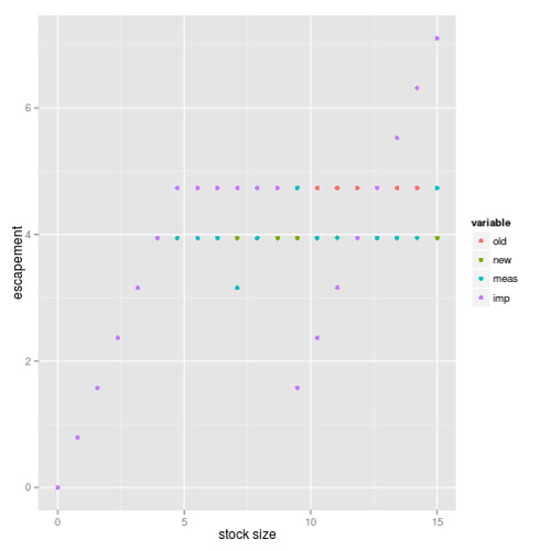
Updated Edit
