Stability analysis on fished and unfished dynamics.

In this example, we compute the distribution of the stability coefficients estimated from the fished and unfished simulations. Overall this shows little success in distinguishing between the stability of the fished and unfished populations – i.e. no hint that we are managing near an edge.

(Originally run and posted in github notebook, but cross posting for reference here since I had trouble recalling if this was filed with the control project or the warning signals project directory. Hence the backdating too.)

Model setup

Clear the workspace and load package dependencies. pdgControl is my implementation of these optimization methods and should be installed from this repository, see README.

Define basic parameters of the economic optimal control problem. We have a discrete economic discounting rate, and will solve the dynamic problem over a time window of 50 years. In the discrete implementation we do not inforce the boundary condition, but rather put a value on meeting it. The optimal solution may choose to not statisfy this boundary condition if the benefit outways this lost reward.

delta <- 0.1      # economic discounting rate
OptTime <- 50     # stopping time
reward <- 1       # bonus for satisfying the boundary condition

Use log-normal noise functions for growth noise, measurement error in the stock assessment, and implementation error, following the notation and definitions in Sethi et al. (2005). To begin, we will allow only noise in growth, as in Reed 1979.

sigma_g <- 0.2    # Noise in population growth
sigma_m <- 0.     # noise in stock assessment measurement
sigma_i <- 0.     # noise in implementation of the quota
z_g <- function() rlnorm(1,  0, sigma_g) # mean 1
z_m <- function() rlnorm(1,  0, sigma_m) # mean 1
z_i <- function() rlnorm(1,  0, sigma_i) # mean 1

Chose the state equation / population dynamics function to have alternate stable states. This is a Beverton-Holt like model with an Allee effect, a model based off of Myers et al. (1995). Note here we’re just loading the function from the package. The equilibrium value K is calculated explicitly from the model given this choice of parameters, as is the allee threshold. We’ll use the allee threshold as the final value xT. We’ll start the model at the unharvested stochastic equilbrium size.

f <- Myer_harvest
pars <- c(1, 2, 6) 
p <- pars # shorthand 
K <- p[1] * p[3] / 2 + sqrt( (p[1] * p[3]) ^ 2 - 4 * p[3] ) / 2
xT <- p[1] * p[3] / 2 - sqrt( (p[1] * p[3]) ^ 2 - 4 * p[3] ) / 2 # allee threshold
x0 <- K - sigma_g ^ 2 / 2 

We define a profit function with no stock effect for simplicity. Profit is just linear in price, with some operating cost (which prevents strategies that put out more fishing effort than required when trying to catch all fish.)

profit <- profit_harvest(price_fish = 1, 
                         cost_stock_effect = 0,
                         operating_cost = 0.1)

We solve the system numerically on a discrete grid. We’ll consider all possible fish stocks between zero and twice the carrying capacity, and we’ll consider harvest levels at the same resolution.

gridsize <- 100   # gridsize (discretized population)
x_grid <- seq(0, 2 * K, length = gridsize)  

h_grid <- x_grid  

The perfect policy

Having defined the problem, we are now ready to calculate the optimal policy by Bellman’s stochastic dynamic programming solution. We compute the stochastic transition matrices giving the probability that the stock goes from any value on the grid x at time t to any other value y at time t+1, for each possible harvest value. Then we use this to compute the optimal harvest rate at each time interval in the system, solving backwards by dynamic programming. The functions to do this are implemented in this package.

SDP_Mat <- determine_SDP_matrix(f, pars, x_grid, h_grid, sigma_g )
opt <- find_dp_optim(SDP_Mat, x_grid, h_grid, OptTime, xT, 
                     profit, delta, reward=reward)

The implementation

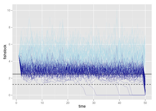
Here we see how this policy performs over 100 replicates

sims <- lapply(1:100, function(i){
  ForwardSimulate(f, pars, x_grid, h_grid, x0, opt$D, z_g, z_m, z_i)
})

Outcome

We summarize the results of the simulation in a tidy data table.

dat <- melt(sims, id=names(sims[[1]]))  

dt <- data.table(dat)
setnames(dt, "L1", "reps") # names are nice





crashed <- dt[time==as.integer(OptTime-1), fishstock < xT, by=reps]
setkey(dt, reps)
setkey(crashed, reps)
dt <- dt[crashed]
setnames(dt, "V1", "crashed")

p1 <- ggplot(dt) + geom_abline(intercept=opt$S, slope = 0) + 
  geom_abline(intercept=xT, slope = 0, lty=2) 
p1 + geom_line(aes(time, fishstock, group = reps), alpha = 0.2, col="darkblue") + 
 geom_line(aes(time, unharvested, group = reps), alpha = 0.2, col="lightblue")  

Stability calculations

Define a quick function to return just the parameters (or missing values if algorithm does not converge).

require(earlywarning)
stability <- function(x){
  n <- length(x)
  x <- x[1:(n-2)]
  fit <- stability_model(x, "OU")
  if(fit$convergence)
    out <- as.list(fit$pars)
  else
    out <- as.list(rep(NA, length(fig$pars)))
  out
}

This function can then be applied to the variable in the data.table.

fished = dt[!crashed, stability(fishstock), by=reps]
unfished = dt[!crashed, stability(unharvested), by=reps]

We can then plot the resulting distribution of parameters. (Annoyingly we have to reformat the data to get it in tidy form again).

# tidy format, columns are variables: rep, variable, value, type





unfished_d <- melt(data.frame(cbind(unfished, type="unfished")), id=c("reps", "type"))
fished_d <- melt(data.frame(cbind(fished, type="fished")), id=c("reps", "type"))
dat <- rbind(fished_d,unfished_d)
ggplot(dat) + geom_boxplot(aes(variable, value, fill=type))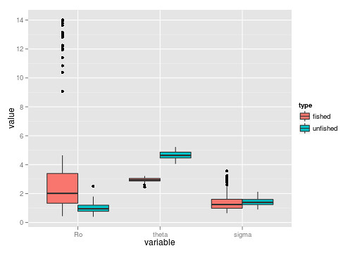 

ggplot(dat, aes(value, variable)) + geom_ribbon(aes(ymax = ..density.., ymin=-..density..),  stat="density") + facet_grid(variable ~ type, as.table=FALSE, scales="free_y")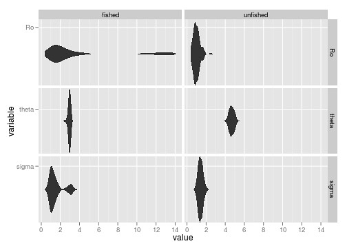 

It’s not entirely evident that we have bimodal distributions from the boxplots. The beanplot (perversion of ggplot’s ribbon plot) makes this abundantly obvious.

So what are those outliers doing?

weirdos <- fished$reps[fished$Ro>10]
ggplot(subset(dt, !(reps %in% weirdos) )) +
  geom_line(aes(time, fishstock, group=reps), alpha=.7) +
  geom_line(dat=subset(dt, (reps %in% weirdos)),
            aes(time, fishstock, group=reps), col="purple", alpha=.4)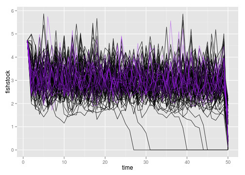

If anything they are less variable, but not exceptionally so. Likely this is estimation error.

mean(dt[reps %in% weirdos,var(fishstock), by="reps"]$V1)

[code][1] 0.5116

```

mean(dt[!(reps %in% weirdos),var(fishstock), by="reps"]$V1)

[code][1] 0.6191

```

Note that the populations do not show different coefficients of variation:

f1 <- dt[,var(fishstock)/mean(fishstock), by=reps]$V1
f2 <- dt[,var(unharvested)/mean(unharvested), by=reps]$V1
mean(f2)

[code][1] 0.2306

```

mean(f1)

[code][1] 0.2239

```