Manuscript revisions
- Heard back from Alan this morning on manuscript, need to cut wordcount in half, from 3000 to 1500 words.
- Should emphasize the countless and utterly arbitrary choices made in every one of these analyses.
- Should emphasize our approach can be applied without replicates. (also without interpolating/having evenly sampled data)
- Should do coefficient of variation on non-detrended data(?) should discuss?
Chemostat data
This morning Alan sent me the data used by Drake & Griffen (Drake & Griffen, 2010). Step one: reread Drake & Griffen.
Notes on reading
- Based on hypothesized transcritical bifurcation. Data does not show the pattern expected by transcritical bifurcation though – mean should stay constant as the value of r changes in the logistic model, and yet they emphasize finding a change in this as if that is expected (i.e. Figure 1b inset). And then they decide not to detrend. Meanwhile Scheffer paper uses saddle-node example in which the mean should change and they assume it should not, and do detrend. All backwards.
- Main article uses only ensemble data over 30 deteriorating environment and 30 from the control group.
- Note they also use a composite index – despite the fact that everything except CV is wrong more often then it is right (see supplement)
- Detrending subtracts a loess smooth instead of kernel smoothing. They use the raw (non-detrended data) after showing it has a better classification rate. Ok for a “best case” test, but rather poor statistical form to pick whatever method gets the highest “correct” rate.
- So how do the classify a warning signal? They start deteriorating the environment after some time interval into the experiment (to remove transients). They estimate the likely point of the bifurcation (without any treatment of uncertainty). They calculate the warning signal over this interval of 16 data points, then take “any increase or local maximum” in this window. (sliding window size of 8 points).
From the supplement
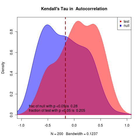
Table A1 shows false positive and false negative rates on the individual runs after classification. Almost all individual runs are classified as no-warning. CV has a 2:3 chance of catching the warning signals in the collapsing group, other stats do worse than random.
Replicating Results
All results can be rerun, generating the plots again, by executing main.R. Caution, produces too many plot windows and errors.
Open main.R, run the library loads, source preprocess.R and ensembles.R
Reanalysis: Independently exploring data
Applying my methods to a single replicate from a warning signals example: (see code)
    id <- det.set$ID[1]
      w<-8   #size of moving window in terms of sampling periods
      pop<-data.frame(day=populations$day[populations$ID==id],x=populations$x[populations$ID==id])
      pop<-pop[order(pop$day),]

    interval <- pop$day > 154 & pop$day < 271
    X <- pop[interval,]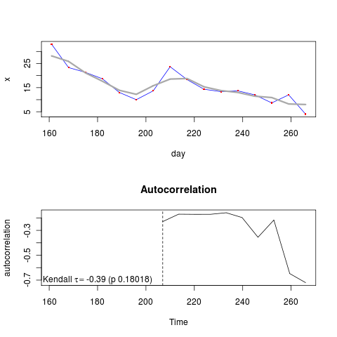
No real hope of detecting a warning signal in this example. Applying my method to the ensemble average data, need to group first by day – will have to figure out how to do this, differs in syntax between methods, i.e.,
    cv.det<-aggregate(timeseries$y[timeseries$Deteriorating==1],by=list(day=timeseries$day[timeseries$Deteriorating==1]),cv)
    ## while skew requires a bit more prep
    det.set<-data.frame(ID=unique(timeseries$ID2[timeseries$Deteriorating==1]),deteriorating=1)
    const.set<-data.frame(ID=unique(timeseries$ID2[timeseries$Deteriorating==0]),deteriorating=0)
    deteriorating<-rbind(det.set,const.set)
    populations<-merge(populations,deteriorating)
    skew.const<-aggregate(populations$x[populations$deteriorating==0],by=list(day=populations$day[populations$deteriorating==0]),skewness)
Note uses skewness from the package “moments,” perhaps a better choice than the moments from the psych package.
Handling Ensembles properly
Having ensemble data, particularly form a test group and control group, provides some unique opportunities.
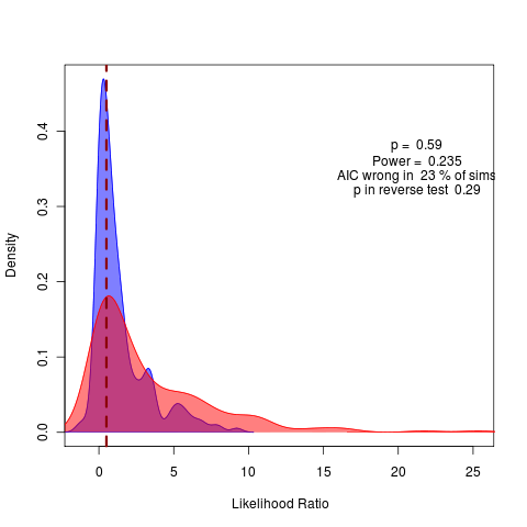
I can draw from these directly, rather than from simulated data, to perform the parametric bootstrap of likelihood-based model fits to illustrate how distinct the data really are relative to their MLE estimates.
I can integrate the approach over datasets: treating each replicate as individual and performing fits, simulation, and posterior re-estimation for model comparisons.
References
- Drake J and Griffen B (2010). “Early Warning Signals of Extinction in Deteriorating Environments.”, Nature. https://dx.doi.org/10.1038/nature09389.