Setting up some adaptive dynamics simulations to complete the parameter-space search. Currently the demo library contains two files, providing the coexistence-only tests and the full evolutionary simulation. This picks up from Aug 30/Sept 1 on coexistence times and Aug 12/13 entrieson waiting times until branching (while still on OWW).
coexistence times
coexist_times.R creates contour plots of the coexistence time under demographic noise expected at a particular position of the pairwise invasibility plot (PIP). I also attempt to calculate these using an analytic approximation derived through the Arrhenius law trick to the SDE approximation.
ensemble_coexistence() runs just the coexistence simulation from
coexist_analytics() attempts to create the same graph analytically.
Unfortunately the analytic approximation seems insufficient:
[flickr-gallery mode =“tag” tags=“contour_analytics_vs_simulation”]
Phases of the branching Process
ensemble_sim() runs the full simulation with mutations. Returns an ad_ensemble object with three elements: $data, $pars, and $reps. $data is a list element for each replicate. For each replicate, it records 4 time-points:
First time two coexisting branches are established
Last (most recent) time two coexisting branches were established
Time to finish phase 2: (satisfies invade_pair() test: trimorphic, third type can coexist (positive invasion), is above threshold and two coexisting types already stored in pair
Time to Finish line (a threshold separation): traits separated by more than critical threshold
For each of these it returns the trait values of the identified coexisting dimorphism as well (x,y). This x,y data is plotted for all replicates in four butterfly plots (for each time interval) by plot_butterfly. Time data is coded in the shading. (just call plot_butterfly on the ad_ensemble object).
In addition to these four (t, x, y) triplets, each replicate reports two counts:
Number of times the dimporphism is lost in phase 2
Number of times the dimorphism is lost in phase 1
These are histogrammed by plot_failures(object). Finally, plot_waitingtimes(object) just histograms the distribution of waiting times across replicates for each of the four phases outlined above. Figures from today’s version of waiting_times.R
[flickr-gallery mode=“tag” tags=“waiting_times”]
Illustrating Key Phenomena
The motivation for these two lines of investigation go back to simulations from May 3-4 entries which begin to show distinction between different mechanisms of branching. The hint comes between processes that appear limited by phase 1 an those limited by phase 2. This can be illustrated by the time required or the number of attempts necessary (failure rate histograms).
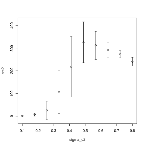
Running simulation sets now varying the range of sigma_mu, sigma_c2, and mu to illustrate the sharpness of the transitions between noise-limited and not limited branching dynamics, and how the difference in times and attempts between phases changes with these parameters. i.e.
Computing Notes:
Setup AdaptiveDynamics repository on zero. An outdated rsa_id key in /.ssh was causing me not to be able to commit from