I’ve been thinking about a few elements of the Monte Carlo approach that seem to be particularly subtle in interpretation. Thought I’d write them out here as a separate examples to help think through them. Thoughts?
Question 1
Should the Monte Carlo simulations use the maximum likelihood test and null model estimated from the data (as in McLachlan 1987, Goldman 1993, Huelsenbeck 1996) or draw from the distribution of model parameters for each simulation?
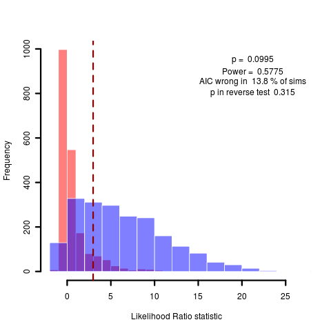
Sometimes this estimate is very uncertain, which is only subtly displayed in the Monte Carlo comparison. While the summary statistics don’t catch it, the graph shows a huge range of likelihood ratios produced when simulating under the test model. Consider the figure below comparing the pure BM model to one with reduced phylogenetic signal (lambda model). Some of the simulations correspond to cases where the MLE estimates a very distinctly different value of lambda (near zero, say), and the model is easy to tell from BM (equivalent to lambda=1). This gives the high likelihood ratios seen on the far right. However, other simulations are very hard to tell apart because they are estimating values of lambda that are very close to unity already.
(code)
The danger is this: that the MLE returns a value of lambda near unity, and the lack of power is attributed to the fact that the data appears nearly Brownian, when in fact considerable lack of power may remain on this data set even if the estimate were near zero. It is in this kind of example that the complete power curves are particularly crucial. As an example, here’s the power curve on lambda for the anoles data:
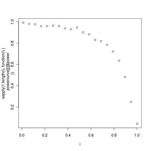
(c0de) The individual distribution at each point can be seenin this series:
[flickr-gallery mode=“tag” tags=“powercurve4”]
question 2
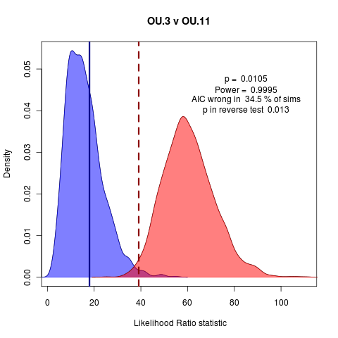
Is the better model the one with the smallest type I error in rejecting the other (integrating under the tail away from the observed likelihood ratio) or the model under which the observed likelihood ratio is most probable?
(code)
The above example (OU.3 v OU.11, see near end of code file) doesn’t quite capture this, since the better p value rejects the null and the higher probability at the observed ratio corresponds to the test distribution, so the methods agree, just. It’s not obvious which one makes the better argument. It is easy to imagine in a borderline case such as this that it could have gone either way though, with the probability being slightly higher or the tail slightly longer.
A related curiosity: would it be useful to estimate a metric of distance between the distributions (maybe Kulback-Leibler divergence, restoring a modern information theoretic feel to it) then the power estimate (although that has a tighter interpretation as Type II error probability)?