On Post-predictive Verification
Considering the kind of post-predictive verification I was discussing with Dan on Tuesday. Let’s start with the simple birth-death branching process. Starting from the master equation, the linearity gives us an accurate model as a Gaussian process where the systematic van Kampen expansion gives us the Fokker Planck equation whose solution is completely specified by its first two moments:
[latex] = (- ) N \
= (- ) ^2 ++
Excellent. So the probability of N species after time t is given by a Gaussian with mean $ N_0 e^{(-)t} $ and variance
\[ \frac{\lambda+\mu}{\lambda-\mu} \left(e^{\alpha t} - 1\right) + N_0 e^{\alpha t}/\alpha - \gamma \]
So we’re interested in the likelihood, i.e. the probability of $ P(| N) $, for simplicity let $ = 0$ for the moment. The expected value is just $ N = N_0 e^{t} $ so that $ = (N/N_0)/t $. Meanwhile, the maximum likelihood estimator for $$ is the maximum of the above expression. We can calculate this analytically in closed form,(help from wxmaxima).
\[ \hat \lambda = \log\left( \frac{\sqrt{4 N_o^4-8 N_0^3N+ 4N_0^2N^2+1}}{2N_0^2}-\frac{1}{2N_0^2} +1\right)/t \]
Which can be rewritten in terms of $ N/N_0$.


Observe that this maximum likelihood value is strictly less than the expected value, i.e. solving in case $ N_0 = 1$ (need to clean chalkboard!)
\[ \frac{\log\left( \frac{\sqrt{4\,{N}^{2}-8\,N+5}}{2}+\frac{1}{2}\right) }{t} \]
Also note though that the expected and maximum likelihood estimates agree in the reasonable limit $ N N_0$. The analytics are presumably closed form but far less tractable with $ $ 0$. Will need to explore the extent of this possible disagreement further later… Also have some exploratory code on this in rabosky_test.R in github.
Generalizing the Codebase
Currently have focused on models fitted through the OUCH software. The format of the power_between_models function in powertest.R fails to generalize immediately only because ouch fits are proper fit objects that have methods like simulate and update already associated with them, and store their likelihood value in the S4 class format under object@loglik. If the fits from geiger, etc, were modified to recognize the standard general methods, they’d work just as well in this routine. Should certainly look into generalizing them, as it would be interesting to start applying the Monte Carlo approach to more methods.
Back to Likelihood paper…
Wondering if it is worth including the all-unique example. Also should include BM vs OU.1 (has OUCH’s funny habit of the extra penalty on OU.1, as it doesn’t estimate the root state), BM vs OU.3 (formerly OU.LP). Adding to the manuscript simulation collection.
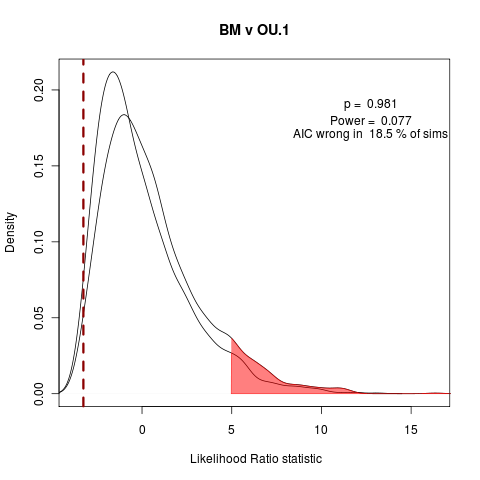
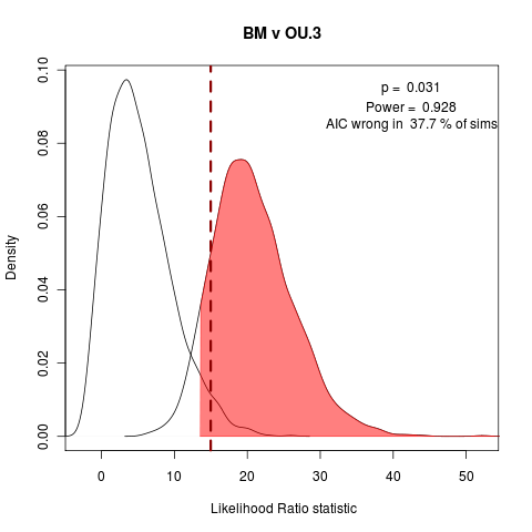
Quick look at AIC fraction of wrong answers in the simulations under each of the following model comparisons:
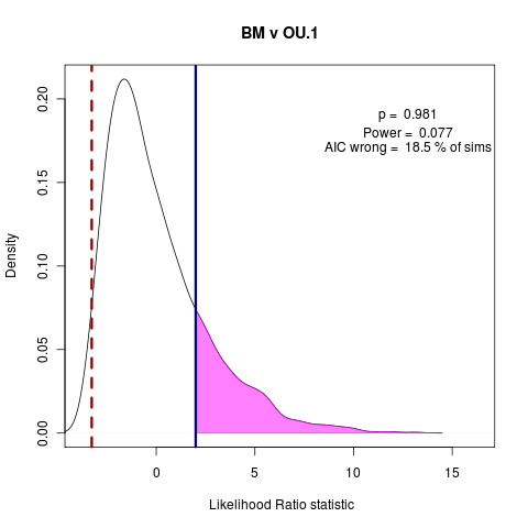
> png("bm_v_ou1.png")
> plot(bm_v_ou1, test_dist=F, shade_p=F, shade_power=F, show_aic=T, shade_aic=T, main="BM v OU.1")
[1] "AIC prefers null model"
[1] "p = 0.981 , power = 0.077"
> dev.off()
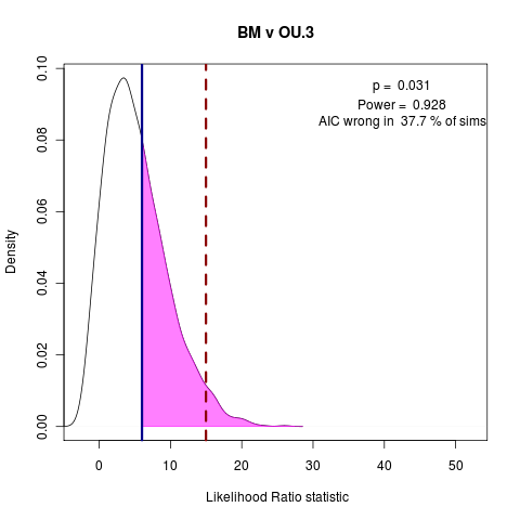
> png("bm_v_ou3.png")
> plot(bm_v_ouLP, test_dist=F, shade_p=F, shade_power=F, show_aic=T, shade_aic=T, main="BM v OU.3")
[1] "AIC prefers test model"
[1] "p = 0.031 , power = 0.928"
> dev.off()
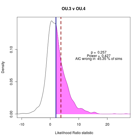
> png("ou3_v_ou4.png")
> plot(ouLP_v_ouLP4, test_dist=F, shade_p=F, shade_power=F, show_aic=T, shade_aic=T, main="OU.3 v OU.4")
[1] "AIC prefers test model"
[1] "p = 0.257 , power = 0.427"
> dev.off()And a look at the power in each of these cases
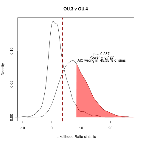
The vastly over-parameterized all-diff model has convergence issues, not surprisingly… Will probably focus on these three comparisons, moving into the power curve discussion.