Recall that we consider the power spectrum of some measurable fluctuating quantity x(t), defined as
\[ y(\omega) = \int_0^T dt e^{i\omega t} x(t) \] \[ S(\omega) = \lim_{T \to \infty} \frac{1}{2\pi T} \left| y(\omega)\right|^2 \]
A little work can show is equal to the Fourier transform of the autocorrelation function, $ x(t) x(t’) = C(t-t’) $.
We evaluate the correlation function of their Fourier transform (note $ x () $ is really $ x()$, the new transformed variable, I’ve dropped the tilde only out of laziness):
\[ \langle x(\omega) x(\omega') \rangle = \langle \int dt e^{i\omega t} x(t) \int dt' e^{i\omega' t'} x(t') \rangle \]
Bringing the expectation inside (by linearity) \[ \int dt \int dt' e^{i(\omega t+\omega' t')} \langle x(t) x(t') \rangle \]
Defining $ = t-t’$, using the definition of the correlation function we have \[ \int dt e^{i (\omega+\omega') t'} \int d \tau e^{-i \omega' \tau} C(\tau) \]
And we see that the $ t $ integral is the (two pi times the) delta function, hence\[ \langle x(\omega) x(\omega') \rangle = 2 \pi \delta (\omega + \omega') \int d \tau e^{i \omega \tau} C(\tau) \]
Note that in the last step we use the fact that delta fn is zero except where $ = -’$, and we define this last integral as the Power spectrum, $ S()$. Noting that as it is complex, $ x(-) = x(^*) $, so
\[ \langle x(\omega) x^*(\omega' ) \rangle = 2\pi \delta(\omega -\omega') S(\omega) \],
or at $ = -$, we have as claimed:
\[ \langle x(\omega) x^*(\omega) \rangle = 2\pi S(\omega) \].
Which is known as the Weiner Khinchine theorem. Time averaging over the stationary distribution instead of averaging across replicates gets us the above version. Getting this to work in the code has been less than successful.
A canonical example: our OU process case
For the OU process, we can write down the correlation function of the stationary distribution (or even the time-dependent solution if we wanted) directly from an application of the the Ito calculus, (see OU solution),
\[ C(\tau) = \frac{\sigma^2}{2\alpha} e^{-\alpha |\tau|} \],
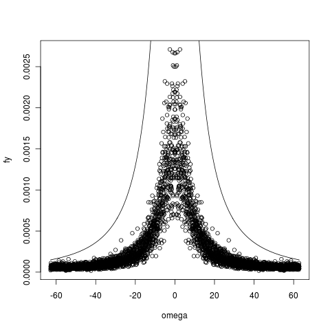
We can compute the Fourier transform of this analytic solution by hand, and recover the Lorentzian curve,
\[ S(\omega) = \frac{\sigma^2}{\alpha^2 +\omega^2} \]
Troubles
I seem to be having difficulty demonstrating this in the simulation.:
Several practical concerns and options:
Accurate simulation of the OU process. As we know the solution, this can be simulated exactly. I’ve explored simulating it through simple Euler, the exact simulation, the analagous discrete time AR(1) process, and the general Milstein regime from the SDE R package. Some differences, particularly visible in Euler vs exact, in the power spectrum, but neither lining up perfectly with the theoretical curve above.
Discussion of normalization. The above Lorentzian is not normalized to integrate to unity, actually equals $ ^2/ $. However this should reflect the actual power calculated from the system above.
Discretization concerns. Long enough T, small enough dt, N, normalizing, rescaling, averaging, Nyquist frequency.
Fourier definition concerns. The definition can differ by a factor of 2 pi between physics and engineers. Further, getting the units of the x-axis correct to line up frequencies with the correct components of the transform is crucial. As a quick check I confirm that the fft of a sine function gives me the peak at the angular frequency I expect:
n<- 2^10 dt<-1/8 t <- seq(0,dt(n-1), by=dt) X <- sin(5t) + rnorm(n, .01) pwr <- abs(fft(dtX))^2/(2pidtn) nyquist<-1/(2dt) # half the sampling frequency w <- nyquistseq(0, 2*pi, length=n/2) plot(w, pwr[1:(n/2)], type=“l”) abline(v=5, col=“red”, lty=3)

Anyway, still in the troubleshooting process, trying to keep exploration documented in the version commits of power_spec.R, so see code and commit log.
Some other notes
If we define the Power spectrum as the transform of $ C()$, then the inverse transform gives us (in Physics convention for Fourier)
\[ C(\tau) := \langle x(t) x(t') \rangle = \int_{-\inf}^{\inf} \frac{d \omega}{2 \pi} e^{-i \omega (t-t')} S(\omega) \]
and setting $ t = t’$ we have
\[ \langle [x(t) ]^2 \rangle = \int_{-\infty}^{\infty} \frac{d \omega}{2 \pi} S(\omega) \]
Now if x(t) is Gaussian process, we can look at the transform of the errors. We note the transform of the Gaussian is Gaussian, taking the function that is normally distributed in x with variance $ ^2$ to one normally distributed in $ $ with variance $ /^3 $.