Semi Analytic Posteriors

The difficulty in comparing the nonparametric Bayesian inference against parametric Bayesian inference is ensuring that the poorer performance of the latter is not do to numerical limitations of the MCMC (no one is quite so worried about the cases where the mcmc solution appears to work well…) Convergence is almost impossible to truly establish, and lots of pathologies (correlations between variables, particularly without simulataneous updating) can frustrate it considerably. While multiple chains and long run times are the reasonable default, for simple enough models we can take a more direct approach.

• Script matches commit 26d84c/semi-analytic-posteriors.md

Generating Model and parameters

Ricker model, parameterized as

\[X_{t+1} = X_t r e^{-\beta X_t + \sigma Z_t}\]

for random unit normal \(Z_t\)

f <- function(x,h,p)  x * p[1] * exp(-x * p[2]) 
p <- c(exp(1), 1/10)
K <- 10  # approx, a li'l' less
Xo <- 1 # approx, a li'l' less

sigma_g <- 0.1
z_g <- function() rlnorm(1,0, sigma_g)
x_grid <- seq(0, 1.5 * K, length=50)
N <- 40
set.seed(123)

Sample Data

x <- numeric(N)
x[1] <- Xo
for(t in 1:(N-1))
  x[t+1] = z_g() * f(x[t], h=0, p=p)
qplot(1:N, x)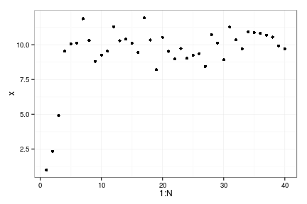

Compute the posterior after marginalizing over \(r\) and \(\sigma\) parameters:

\[P(\beta | X) \]

Mt <- function(t, beta) log(x[t+1]) - log(x[t]) + beta * x[t]
beta_grid = seq(1e-5, 2, by=1e-3)

P_B.X <- sapply(beta_grid, function(beta){
  Mt_vec = sapply(1:(N-1), Mt, beta)
  sum_of_squares <- sum(Mt_vec^2)
  square_of_sums <- sum(Mt_vec)^2
  0.5 ^ (N/2-1) * (sum_of_squares - square_of_sums/(N-1)) ^ (N/2-1) / gamma(N/2-1)
  })

qplot(beta_grid, -log(P_B.X))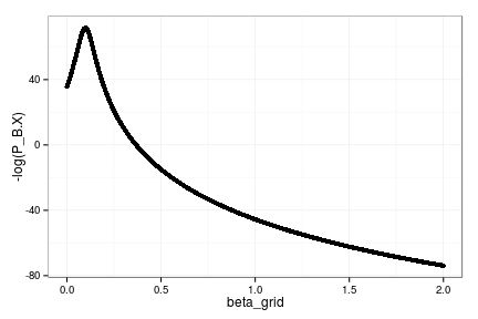

Posterior mode is at:

beta_grid[which.min(P_B.X)]

[1] 0.09801

Estimating the Myers model on this data:

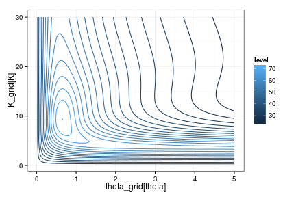
\[X_{t+1} = Z_t \frac{r X_t^{\theta}}{1 + X_t^{\theta} / K}\]

With \(Z_t\) lognormal, unit mean, std \(\sigma\).

Marginal distribution over the remaining parameters is a 2D grid:

Mt <- function(t, theta, K) log(x[t+1]) - theta * log(x[t]) + log(1 + x[t] ^ theta / K) 
theta_grid = seq(1e-5, 5, length=100)
K_grid = seq(1e-5, 30, length=100)

prob <- function(theta, K){
  Mt_vec = sapply(1:(N-1), Mt, theta, K)
  sum_of_squares <- sum(Mt_vec^2)
  square_of_sums <- sum(Mt_vec)^2
  0.5 ^ (N/2-1) * (sum_of_squares - square_of_sums/(N-1)) ^ (N/2-1) / gamma(N/2-1)
}



P_theta_K.X <- sapply(theta_grid, function(theta)
                sapply(K_grid, function(k) prob(theta, k)))


require(reshape2)

df = melt(P_theta_K.X)
names(df) = c("theta", "K", "lik")
ggplot(df, aes(theta_grid[theta], K_grid[K], z=-log(lik))) + stat_contour(aes(color=..level..), binwidth=3)