Running into some unpredictable and not consistently replicable memory errors in the tgp function calls. Also rather troublesome that return object provides only posterior means for the process mean and covariance matrix.
Generic GP methods
- Implemented MCMC sampler. Excerpt below based on my gaussian-process-basics.md script, as updated to include this case.
Define some example priors
lpriors <- function(pars){
   d.p <- c(5, 5)
  s2.p <- c(5, 5)

  prior <- unname(
    dgamma(exp(pars[1]), d.p[1], scale = d.p[2]) *
    dgamma(exp(pars[2]), s2.p[1], s2.p[2])
  )

  log(prior)
}
Define the posterior function for our metropolis sampler
posterior <- function(pars, x, y){

  l <- exp(pars[1])
  sigma.n <- exp(pars[2])

  cov <- function(X, Y) outer(X, Y, SE, l)
  I <- diag(1, length(x))
  K <- cov(x, x)

  loglik <- - 0.5 * t(y) %*% solve(K + sigma.n^2 * I) %*% y -
    log(det(K + sigma.n^2*I)) -
    length(y) * log(2 * pi) / 2

  loglik + lpriors(pars)
}
I do not think we have good conjugate priors we can use in this situation to accomplish Gibbs sampling. Instead we simply MCMC by the Metropolis-Hastings alogrithm,
require(mcmc)
n <- 1e4
out <- metrop(posterior, log(pars), n, x = obs$x, y = obs$y)
out$accept
[1] 0.1509Very good, we want an acceptance rate around 20%, if the literature can be trusted on this account. We then plot transformed and untransformed traces.
postdist <- cbind(index=1:n, as.data.frame(exp(out$batch)))
names(postdist) <- c("index", names(pars))
df <- melt(postdist, id="index")
# TRACES
ggplot(df) + geom_line(aes(index, value)) + facet_wrap(~ variable, scale="free", ncol=1)
ggplot(df) + geom_line(aes(index, log(value))) + facet_wrap(~ variable, scale="free", ncol=1)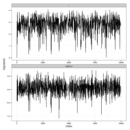
Generate a plot to compare priors and posteriors
d.p <- c(5, 5)
s2.p <- c(5, 5)

s2_prior <- function(x) dgamma(x, s2.p[1], s2.p[2])
d_prior <- function(x) dgamma(x, d.p[1], scale = d.p[2])
prior_fns <- list(l = d_prior, sigma.n = s2_prior)


require(plyr)
prior_curves <- ddply(df, "variable", function(dd){
    grid <- seq(min(dd$value), max(dd$value), length = 100)
    data.frame(value = grid, density = prior_fns[[dd$variable[1]]](grid))
})

# Posteriors (easier to read than histograms)
ggplot(df, aes(value)) +
  stat_density(geom="path", position="identity", alpha=0.7) +
  geom_line(data=prior_curves, aes(x=value, y=density), col="red") +
  facet_wrap(~ variable, scale="free", ncol=2)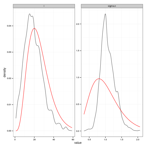
Steve chat
- integrate over posteriors in GP case
- Ignore measurement uncertainty for the moment
- General status updates, etc.
Marc meeting
- Ricker case, but with constraint (e.g. maintain above n%)
- Consider Ricker model with external management constraint $ (Y / Y_opt) + (1 - ) Pr( )$
- Consider time horizon of learning vs implementing; see diagram

Simone talk
General interests: adaptive potential of small pops, demography of small pops, extinction processes in communities, evol life histories & enviroment, ML for species distribution models.
Marble trout system under the influence of regular catastrophic floods
Misc
- 6 hours on trains, 2 hours on buses, 1.25 hours on bicycle, 6 hours in lab.
- Interesting reading in The Secret History of OpenStack, the Free Cloud Software That’s Changing Everything. Sounds just like the unlikely collaboration we need to emerge for a more robust and sustainable underlying scientific infrastructure.