(Corresponds to commit 4bd8422107 in earlywarning repo)
For the individual-based simulation, the population dynamics are given by
\[\begin{align} \frac{dP(n,t)}{dt} &= b_{n-1} P(n-1,t) + d_{n+1}P(n+1,t) - (b_n+d_n) P(n,t), \\ b_n &= \frac{e K n^2}{n^2 + h^2}, \\ d_n &= e n + a, \end{align}\]
which is provided by the saddle_node_ibm model in populationdynamics.
For each of the warning signal statistics in question, we need to generate the distibution over all replicates and then over replicates which have been selected conditional on having experienced a crash.
We begin by running the simulation of the process for all replicates.
Load the required libraries
library(populationdynamics)
library(earlywarning)
library(reshape2)   # data manipulation
library(data.table) # data manipulation
library(ggplot2)    # graphics
library(snowfall)   # parallel
theme_publish <- theme_set(theme_bw(12))
theme_publish <-
theme_update(legend.key=theme_blank(),
panel.grid.major=theme_blank(),panel.grid.minor=theme_blank(),
plot.background=theme_blank(), legend.title=theme_blank())Conditional distribution
Then we fix a set of paramaters we will use for the simulation function. Since we will simulate 20,000 replicates with 50,000 pts a piece, we can save memory by performing the conditional selection on the ones that cross a threshold we go along and disgard the others. (We will create a null distribution in which we ignore this conditional selection later).
threshold <- 250
select_crashes <- function(n){
  T<- 5000
  n_pts <- n
  pars = c(Xo = 500, e = 0.5, a = 180, K = 1000, h = 200,
    i = 0, Da = 0, Dt = 0, p = 2)
  sn <- saddle_node_ibm(pars, times=seq(0,T, length=n_pts), reps=1000)
  d <- dim(sn$x1)
  crashed <- which(sn$x1[d[1],] <= threshold)
# crashed <- which(sn$x1[d[1],]==0)
  sn$x1[,crashed]
}
A few extra commands format the data into a table with columns of times, replicate id number, and population value at the given time.
sfInit(parallel=FALSE)
sfLibrary(populationdynamics)sfExportAll()
examples <- sfLapply(1:20, function(i) select_crashes(50000))
dat <- melt(as.matrix(as.data.frame(examples, check.names=FALSE)))
names(dat) = c("time", "reps", "value")
levels(dat$reps) <- 1:length(levels(dat$reps)) # use numbers for repsggplot(subset(dat, reps %in% levels(dat$reps)[1:9])) + geom_line(aes(time, value)) + facet_wrap(~reps, scales="free")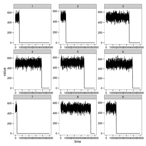
Zoom in on the relevant area of data near the crash
require(plyr)
zoom <- ddply(dat, "reps", function(X){
    tip <- min(which(X$value<threshold))
    index <- max(tip-200,1):tip
    data.frame(time=X$time[index], value=X$value[index])
})ggplot(subset(zoom, reps %in% levels(zoom$reps)[1:9])) + geom_line(aes(time, value)) + facet_wrap(~reps, scales="free")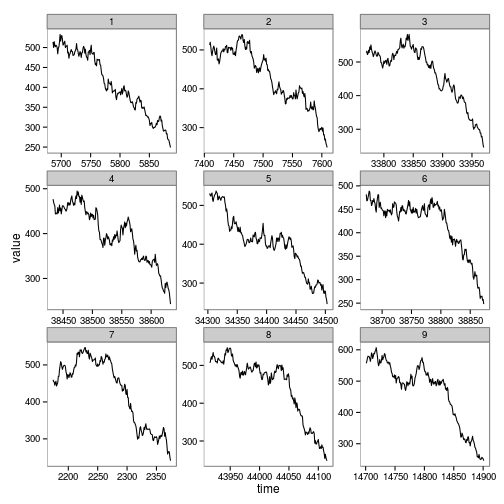
Compute model-based warning signals on all each of these.
dt <- data.table(subset(zoom, value>threshold))
var <- dt[, warningtrend(data.frame(time=time, value=value), window_var), by=reps]$V1
acor <- dt[, warningtrend(data.frame(time=time, value=value), window_autocorr), by=reps]$V1
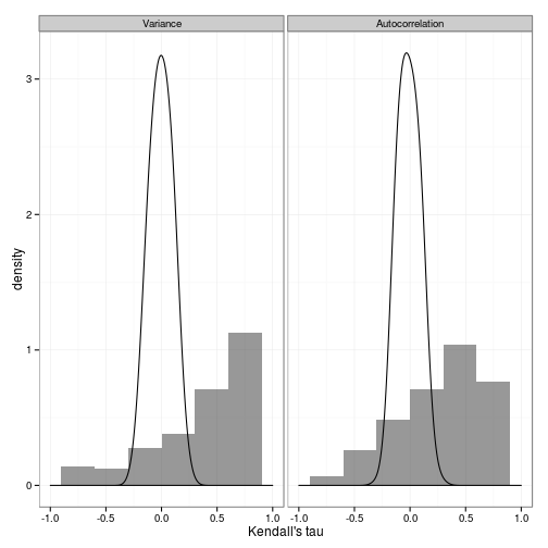
dat <- melt(data.frame(Variance=var, Autocorrelation=acor))Null distribution
To compare against the expected distribution of these statistics, we create another set of simulations without conditioning on having experienced a chance transition, on which we perform the identical analysis.
threshold <- 250
select_crashes <- function(n){
  T<- 5000
  n_pts <- n
  pars = c(Xo = 500, e = 0.5, a = 180, K = 1000, h = 200,
    i = 0, Da = 0, Dt = 0, p = 2)
  sn <- saddle_node_ibm(pars, times=seq(0,T, length=n_pts), reps=500)
  d <- dim(sn$x1)
  sn$x1[1:501,]
}sfExportAll()
examples <- sfLapply(1:10, function(i) select_crashes(50000))
nulldat <- melt(as.matrix(as.data.frame(examples, check.names=FALSE)))
nulldat <- melt(examples)
names(nulldat) = c("time", "reps", "value")
levels(nulldat$reps) <- 1:length(levels(dat$reps)) Zoom in on the relevant area of data near the crash
require(plyr)
nullzoom <- ddply(nulldat, "reps", function(X){
    data.frame(time=X$time, value=X$value)
    })
nulldt <- data.table(nullzoom)
nullvar <- nulldt[, warningtrend(data.frame(time=time, value=value), window_var), by=reps]$V1
nullacor <- nulldt[, warningtrend(data.frame(time=time, value=value), window_autocorr), by=reps]$V1
nulldat <- melt(data.frame(Variance=nullvar, Autocorrelation=nullacor))ggplot(dat) + geom_histogram(aes(value, y=..density..), binwidth=0.3, alpha=.5) +
facet_wrap(~variable) + xlim(c(-1, 1)) +
geom_density(data=nulldat, aes(value), adjust=2) + xlab("Kendall's tau") + theme_bw()