This example goes through the steps to demonstrate that in a sufficiently-frequently sampled timeseries, autocorrelation does contain some signal of early warning. ((Post markdown generated automatically from knitr.))
Run the individual based simulation
require(populationdynamics)[code] Loading required package: populationdynamics
```
pars = c(Xo = 730, e = 0.5, a = 100, K = 1000,
    h = 200, i = 0, Da = 0.09, Dt = 0, p = 2)
time = seq(0, 500, length = 500)
sn <- saddle_node_ibm(pars, time)
X <- data.frame(time = time, value = sn$x1)
compute the observed value:
require(earlywarning)[code] Loading required package: earlywarning
```
observed <- warningtrend(X, window_autocorr)fit the models
$ dX = (- X) dt + dB_t $
$ dX = _t (- X) dt + (_t+) dB_t $
A <- stability_model(X, "OU")
B <- stability_model(X, "LSN")
simulate some replicates
reps <- 100
Asim <- simulate(A, reps)
Bsim <- simulate(B, reps)
tidy up the data a bit
require(reshape2)
Asim <- melt(Asim, id = "time")
Bsim <- melt(Bsim, id = "time")
names(Asim)[2] <- "rep"
names(Bsim)[2] <- "rep"
Apply the warningtrend window_autocorr to each replicate
require(plyr)
wsA <- ddply(Asim, "rep", warningtrend, window_autocorr)
wsB <- ddply(Bsim, "rep", warningtrend, window_autocorr)
And gather and plot the results
tidy <- melt(data.frame(null = wsA$tau, test = wsB$tau))
names(tidy) <- c("simulation", "value")
require(beanplot)
beanplot(value ~ simulation, tidy, what = c(0,
    1, 0, 0))
abline(h = observed, lty = 2)
require(ggplot2)
roc <- roc_data(tidy)[code] Area Under Curve = 0.819680311103255 True positive rate = 0.33 at false positive rate of 0.05
```
ggplot(roc) + geom_line(aes(False.positives, True.positives),
    lwd = 1)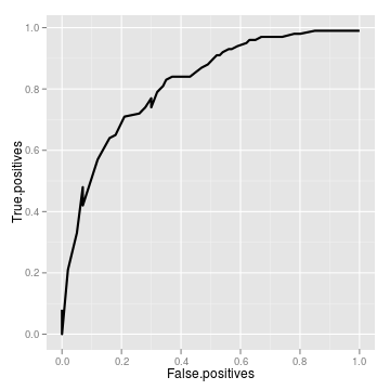
Parallelization
Parallel code for the plyr command is straight-forward for multicore use,
require(doMC)
registerDoMC()
wsA <- ddply(Asim, "rep", warningtrend, window_autocorr,
    .parallel = TRUE)
wsB <- ddply(Bsim, "rep", warningtrend, window_autocorr,
    .parallel = TRUE)
Which works nicely (other than the progress indicator finishing early).
In principle, this can be parallelized over MPI using an additional function, seems to work:
library(snow)
library(doSNOW)
source("../createCluster.R")
cl <- createCluster(4, export = ls(), lib = list("earlywarning"))
ws <- ddply(Asim, "rep", warningtrend, window_autocorr,
    .parallel = TRUE)
stopCluster(cl)
head(ws)
[code] rep tau 1 X1 0.7886 2 X2 0.6966 3 X3 0.6543 4 X4 0.5251 5 X5 -0.2859 6 X6 -0.3889
```