While the wrightscape package is still in active development, I realize the code base doesn’t contain any introductory examples. So as a first tutorial, here’s a short walk-through of the package. We begin by loading the package and a few useful additional packages:
require(wrightscape} # My package for this analysis
require(auteur) # for the data only
require(maticce) # to create paintings
We’ll load a data set of 233 taxa of primates with their body sizes(REDDING et. al. 2010), kindly provided by Eastman et al.(Eastman et. al. 2011) in the Auteur package. We format this data-set using a wrightscape function, which converts both the tree and the data into the ouch format from the ape/geiger format. (Eventually the conversion step will be automated)
data(primates)
monkey <- format_data(primates$phy, primates$dat)
We just have to create the “painting” indicating which regimes can be treated separately, as in ouch. We do this using several handy functions from thematicce package. Selecting the common ancestor two arbitrarily chosen species from different families of New World monkeys should do the trick to identify the New World clade, Platyrrhini.
## Paint the tree with a transition at New World monkeys
new_world_ancestor <- mrcaOUCH(c("Ateles_belzebuth",
                                 "Leontopithecus_caissara"),
                               monkey$tree)
new_world <- paintBranches(new_world_ancestor, monkey$tree,
                            c("OldWorld", "NewWorld"))
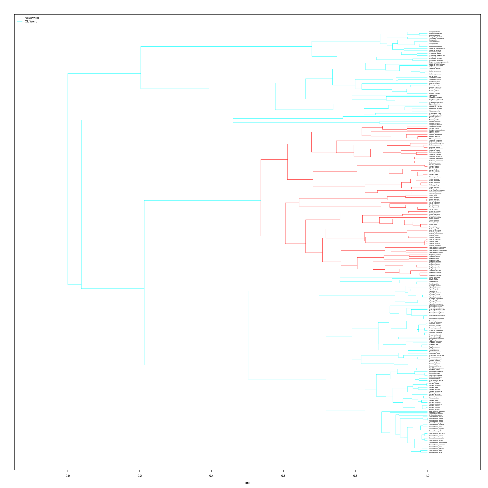
This clade showed a substantially lower rate of body-size evolution in Eastman et al’s RJMCMC analysis under a Brownian model(Eastman et. al. 2011). Now we will test whether that is due to greater stabilizing selection or a greater diversification rate. With the painting and the data, we are ready to construct these wrightscape models.
Wrighstcape uses a general model formulation, of which many common models, such as used by ouch, brownie, and others are subclasses. We can construct these subclasses by fixing certain parameters using the model_spec parameter.
This specifies which parameters out of alpha, theta, and sigma are independently estimated on each regime, kept global across regimes, or, in the case of alpha, fixed to zero (to give purely Brownian behavior). i.e. ouch model is equivalent to: list(alpha=“global”, sigma=“global”, theta=“indep”), while the brownie model is equivalent to list(alpha=“fixed”, sigma=“indep”, theta=“global”).
#####  Estimate the models by maximum likelihood, as in OUCH #####
alphas <- multiTypeOU(data=monkey$data, tree=monkey$tree,
                      regimes=new_world,model_spec =
                      list(alpha="indep",sigma="global",
                      theta="global"), Xo=NULL, alpha = .1,
                      sigma = 40, theta=NULL, method ="SANN",
                      control = list(maxit=100000,temp=50,tmax=20))

sigmas <- multiTypeOU(data=monkey$data, tree=monkey$tree,
                      regimes=new_world, model_spec=
                      list(alpha="fixed", sigma="indep",
                      theta="global"), Xo=NULL, alpha = .1,
                      sigma = 40, theta=NULL, method ="SANN",
                      control=list(maxit=100000,temp=50,tmax=20))
Starting parameter estimates are given or left to NULL. “method” refers to the optimization, using parameters given in control. We’ll use simulated annealing to get a robust result.
The code above estimates a novel model, where only the strength of selection, $ $, has changed in across branches in the OU model:
\[ dX = \alpha_i ( \theta - X) dt + \sigma dB_t \]
While the second example runs a Brownian motion model that differs across regimes:
\[ dX = \sigma_i dB_t \]
Once these have run, we can do a simple comparison by likelihood:
alphas$loglik - sigmas$loglikTo know if this is significant, we would do best to compare the models by PMC (my other package, with upcoming paper):
alphas_v_sigmas <- montecarlotest(alphas, sigmas, cpu=16, nboot=200)
plot(alphas_v_sigmas)
We could instead estimate the posterior distributions by MCMC:
          phylo_mcmc(monkey$data, monkey$tree, new_world,
                     MaxTime=1e5, alpha=.1, sigma=.1,
                     theta=NULL, Xo=NULL, model_spec=
                     list(alpha="indep", sigma="global",theta="global"),
                     stepsizes=0.05)
Of course we would do well to parallelize this call over some large number of nodes to get appropriate mixing.
References
REDDING D, DeWOLFF C and MOOERS A (2010). “Evolutionary Distinctiveness, Threat Status, And Ecological Oddity in Primates.” Conservation Biology, 24. https://dx.doi.org/10.1111/j.1523-1739.2010.01532.x.
Eastman J, Alfaro M, Joyce P, Hipp A and Harmon L (2011). “A Novel Comparative Method For Identifying Shifts in The Rate of Character Evolution on Trees.” Evolution, 65. https://dx.doi.org/10.1111/j.1558-5646.2011.01401.x.