Considering the fits of the quadratic models from yesterday.
[flickr-gallery mode=“tag” tags=“quadraticfitslides” tag_mode=“all”]
Analysis of fits
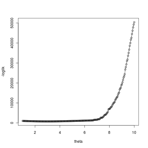
Of course these fits rely entirely on mapping the location of the stable point and the slope through that point, something they still cannot do all that well. In this parameterization the the stable intercept is \[ \hat x = \sqrt{r}+\theta \] and slope at intercept is \[ \frac{\partial f(\hat x)}{\partial x} = -2\sqrt{r} \] This creates a numerical optimization problem, since there is high importance on getting the mean right, and less on the variance, the routine tends to fix the combination of r and theta to get the mean right, and then cannot change r to get the slope correct without getting penalized for the loss of likelihood in changing the mean.
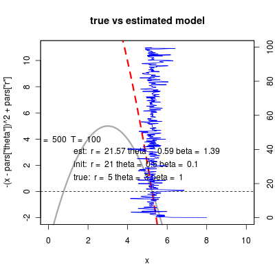
Comparing to estimating linearization provokes a tweak of the model
For this reason would be easier to estimate the OU model directly, and apply the transformation into the equivalent quadratic model.
\[ \theta_{ou} = \sqrt{r}+\theta_{sn} \] \[ \alpha_{ou} = 2\sqrt{r} \] \[ \theta_{sn} = \theta_{ou}- \alpha_{ou}/2 \] \[ r = \alpha_{ou}^2/4 \]
and the variance is slightly more complicated: \[ \frac{ \beta \left(r - (\hat{x}-\theta_{sn})^2 \right)}{2 (\hat x - \theta_{sn} )} = \frac{\sigma^2_{ou}}{2\alpha} \] \] = \[ \[ \beta = \frac{\sigma^2_{ou}\sqrt{r} }{\alpha \left(r - (\hat{x}-\theta_{sn})^2 \right)} \]
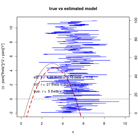
Note that the denominator goes to zero – the SN model as framed above as pure birth has no noise at the equilibrium. Let’s alter this in the simulation, phrased as a birth-death model, perhaps just reversing the sign on the quadratic term, we get a more meaningful:
\[ \beta = \frac{\sigma^2_{ou}\sqrt{r} }{\alpha \left(r + (\hat{x}-\theta_{sn})^2 \right)} \] \[ \beta = \frac{\sigma^2_{ou} }{2 \alpha\sqrt{r} } \]
This implies much larger noise of course, and does seem to provide better estimates. On the right repeated with smaller noise values (see beta parameter estimates).
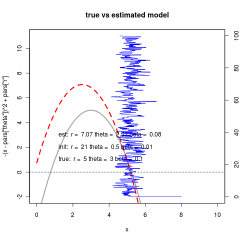
Note that less noise also means less accurate estimate farther out. The Nelder-Meade algorithm is now happy with the convergence:
> out$optim_output$convergence
[1] 0
So how does this compare to estimating by OU?
We estimate the OU model and then infer the quadratic model using the equations derived above:
(code)
So despite the numerical challenges in estimating the quadratic directly, when it can converge it can do quite well; better than the linear fit. This new noise model does much better at handling the case of starting at the far side of the equilibrium, as theta surface is now monotonic since noise doesn’t vanish at the unstable equilibrium:
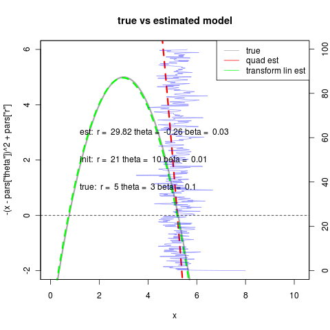
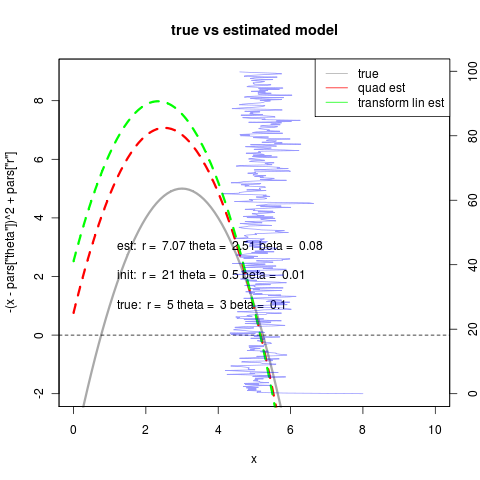
On the right we see that the transformed linear model can still well outperform the quadratic due to the degeneracy we discussed earlier in choosing r and theta (right). In general it may be best to use the linear fitting routine as an initial condition if not as a replacement for the quadratic model.
Model generality
The nice thing about the quadratic formulation (despite having to numerically integrate an ode system instead of use an analytical solution for the conditional probability) is the natural representation of the changing r version in this model.
This doesn’t allow different rates of the bifurcation with change in r. This would require a coefficient to the quadratic, \[ f(x) = r - a(x-\theta)^2 \] \[ \hat x = \sqrt{r/a}+\theta \] \[ \partial f(\hat x) = -2\sqrt{a r} \]
and would be an identifiability issue.