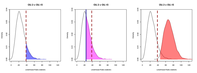
Back to writing for today. Working on discussion of non-nested models. Looking at the reverse comparison, can get the reverse p value. The case of OU.3 vs the OU.4 model doesn’t show either test to be significant at the 95% confidence level,but the case of OU.3 vs OU.15 (lets every species in the top two clades be unique) does:
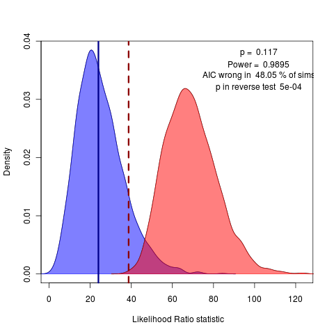
The reverse p value easily rejects this silly OU.15 model, though AIC vastly prefers it. Perhaps this would be a better example to start with then the OU.4 case? Doesn’t have the same convergence issues as the all-diff (OU.23) model, and has a clearer conclusion than the OU.4 choice…
This raises an interesting question though: should a model be preferred because it is rejected in one test and not rejected in the reverse test (at some chosen confidence level), or should it be chosen as the one having the higher likelihood? For instance, these two choices can theoretically disagree:
The curve to the left has a higher probability for the observed LR, but a lower p-value when treated as the null.
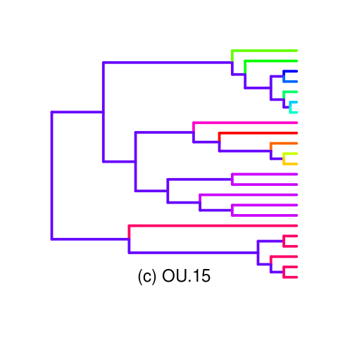
Looking into a clearer opening example such as the OU.15 tree. Wrote a palette function for the tree (inlikelihoodratio_mansucript_examples.R)
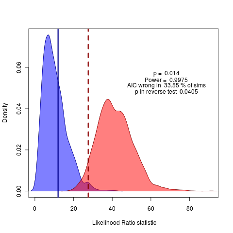
Gives decent example of AIC making the wrong choice, Monte Carlo making a clear different choice, accepting the simpler model with strong degree of information (power).
Unfortunately in this example OU.3 is not nested within this particular painting, even though the ratio is always positive. Making a nested model tends in most examples of over-parameterized models fit neither very well, i.e. this OU.10 model:
see code commit github: ef36d62. Hmm, maybe start with some simpler nested-model comparisons.
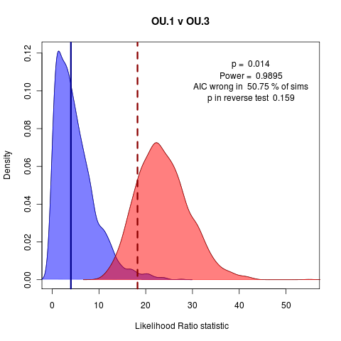
A clear nested case: OU.1 vs OU.3:
Some Simpler Geiger Examples
Currently cannot run on Gieger fits aren’t fit objects. A little wrapper function can get around most of this.
fitContinuous_object <- function(tree, data, model="BM", ...){
    fit <- fitContinuous(tree, data, model=model, ...)
    class(fit) <- "fitContinuous"
    fit$model <- model
    fit$tree <- tree
    fit$data <- data
    fit$root <- phylogMean(fit[[1]]$beta*vcv.phylo(tree), data)
    fit
}
The next problem is the lack of available methods for simulation in Gieger.
I’m afraid that it is ridiculous that sim.char in Geiger ignores the root state under the Brownian motion simulation. Of course it can just be added to the data of the simulation, but no one will do that, or worse, not even realize that the function is ignoring the specification of the root state.
Equally ridiculous is that geiger doesn’t return this estimate of the root state found by fitContinuous, even though it’s estimated from the data and contributes to the fit. It isn’t estimated by the optim function, however, because it can be found independently by estimating from the data directly, as I do in the function above.
Probably faster to extend ouch to optimize over tree transformations. Also avoid the computational drag of Gieger coding. Anyway, just about done, a reasonably object-oriented geiger now. Simulation needs to be extended to perform the tree transformations when required still. See github code.