- Noise in the larval class is damped by
 and grows proportional to its intrinsic variation and the contribution of other classes through their derivatives of fL, that is,
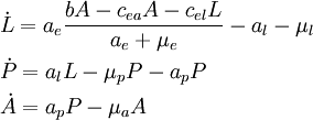
  as well as the sum of its intrinsic rates (essentially whichever is larger). Taking E dynamics to be fast we might reduce to a continous time LPA model:
and the larval fluctuations are essentially:
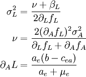
where βi is the intrinsic noise of the age class. Hence a class i which propagates large noise to another class j has a large  . If this term is a linear transition λXi, then the same term appears in fi and hence damps the noise
  and cancels out. Hence noise must propagate into a class through nonlinear transition rates OR through an asymmetry in the transition (i.e. the c_1, c_2 large noise example in the generalized crowley).
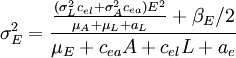
Compare to noise in Eggs:
Adding age delay to beetle dynamics ———————————–
Current formulation has used exponential waiting times between stages. By subdividing the classes (increasing the system dimension size) and creating single jump within-state transitions, these become gamma-distributed waiting times. Adding ten steps to each phase and a little parameter fiddling introduces sustained oscillations. (Version-stable code).
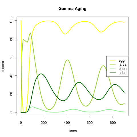
beetle_pars <- c(b=5, ue= 0, ul = 0.001, up = 0.00001, ua = 0.01, ae = 1.3, al = .1, ap = 1.5, cle = .2, cap = .1, cae = 5, V=100)
Xo[1] = 100
- Implementation still needs trouble-shooting, variance dynamics don’t seem to be being computed correctly. done
- Adult class doesn’t need multiple stages. done
- Code should allow for a general k classes rather than a fixed 10 classes. done
and now we have noise in oscillatory, gamma-waiting model:
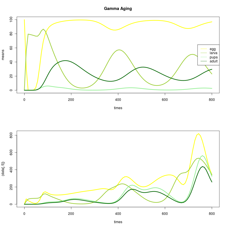
- parameters as before, see version-stable code.
Misc / Code notes —————–
R-evolution parallelizes the variance dynamics calculation (perhaps the matrix multiplication step?) and is probably responsible for the openmp parallelization working.
- article on cloud computing vs grid. reminds me to include questions on cloud computing in the CSGF survey.
Should also take a closer read of the recent: Kendall BE, Wittmann ME. A stochastic model for annual reproductive success. The American naturalist. 2010;175(4):461-8. Available at: https://www.ncbi.nlm.nih.gov/pubmed/20163244.